Introduction
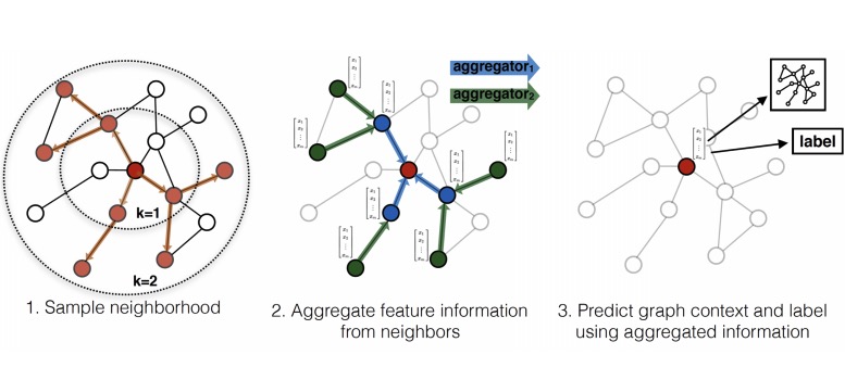
In the previous blogs, we covered GCN and DeepWalk, which are methods to generate node embeddings. The basic idea behind all node embedding approaches, is to use dimensionality reduction techniques to distill the high-dimensional information about a node’s neighborhood into a dense vector embedding. These node embeddings can then be fed to downstream machine learning systems and aid in tasks such as node classification, clustering, and link prediction. Let us move on to a slightly different problem. Now, we need the embeddings for each node of a graph where new nodes are continuously being added. A possible way to do this would be to rerun the entire model (GCN or DeepWalk) on the new graph, but it is computationally expensive. Today we will be covering GraphSAGE, a method that will allow us to get embeddings for such graphs in a much easier way. Unlike embedding approaches that are based on matrix factorization, GraphSAGE leverage node features (e.g., text attributes, node profile information, node degrees) in order to learn an embedding function that generalizes to unseen nodes. GraphSAGE is capable of learning structural information about a node’s role in a graph, despite the fact that it is inherently based on features.
The Start
In the (GCN or DeepWalk) model, the graph was fixed beforehand, let's say the 'Zachary Karate Club', some model was trained on it, and then we could make predictions about a person X, if he/she went to a particular part of the club after separation.

In this problem, the nodes in this graph were fixed from the beginning, and all the predictions were to be made on these fixed nodes only. In contrast to this, take an example where ‘Youtube’ videos are the nodes and assume there is an edge between the related videos, and say we need to classify these videos depending on the content. If we take the same model as in the previous dataset, we can classify all these videos, but whenever a new video is added to ‘YouTube’, we’ll have to re-train the model on the entire new dataset again to classify it. Due to too many videos or nodes being added, it is not computationaly feasible for us to re-train everytime.
To solve this issue, what we can do is not to learn embeddings for each node but to learn a function which, given the features and edges joining this node, will give the embeddings for the node.
Aggregating Neighbours
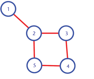
The idea is to generate embeddings, based on the neighbourhood of a given node. In other words, the embedding of a node will depend upon the embedding of the nodes it is connected to. Like in the graph below, the node 1 and 2 are likely to be more similar than node 1 and 5.
How can this idea be formulated?
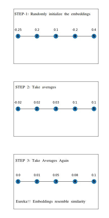
First, we assign random values to the embeddings, and on each step, we will update the value of the embedding using the average of embeddings for all the nodes it is connected to directly .
The following example shows the working on a simple linear graph.
This is a straightforward idea, which can be generalized by representing it in the following way,
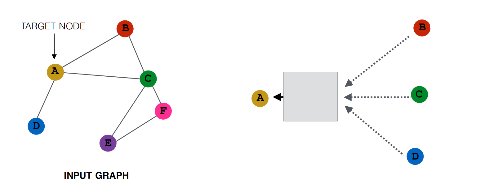
Here The Box joining A with B, C, D represents some function of the A, B, C, D. ( In the animation above, it was the ‘mean’ function). We can replace this box by any function like ‘sum’ or ‘max’. This function is known as the aggregator function.
Now let’s try to generalize the notion by using not only the neighbours of a node but also the neighbours of the neighbours. The first question is how to make use of neighbours of neighbours. The way which we will be using here is to first generate each node’s embedding in the first step by using only its neighbours just like we did above, and then in the second step, we will use these embeddings to generate the new embeddings.
Take a look at the following One Layer Aggregation:
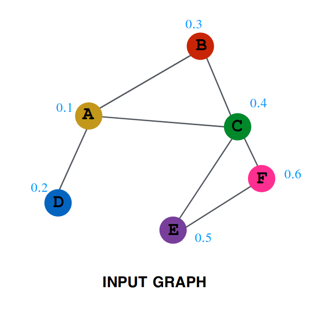
The numbers written along with the nodes are the value of embedding at the time, T=0.
Values of embedding after one step are as follows:

So after one iteration, the values are as follows:
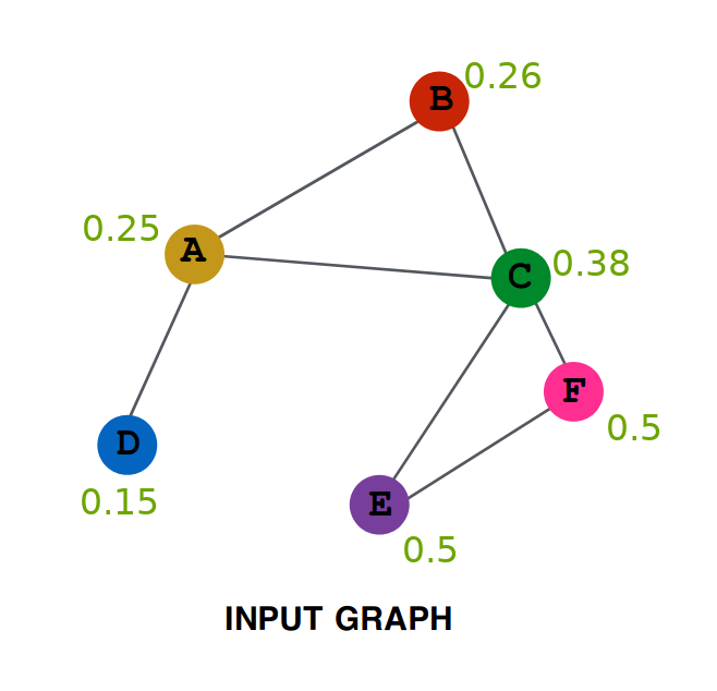
Repeating the same procedure on this new graph, we get (try verifying yourself) Aggregation After Two Layers:
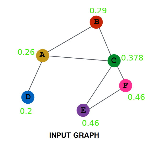
Lets try to do some analysis of the aggregation. Represent by $A^{(0)}$ the initial value of embedding of A ( i.e. 0.1 ), by $A^{(1)}$ the value after one layer ( i.e. 0.25 ) similarly $A^{(2)}$, $B^{(0)}$, $B^{(1)}$ and all other values.
Clearly
$$A^{(1)} = \frac{(A^{(0)} + B^{(0)} + C^{(0)} + D^{(0)})}{4}$$
Similarly
$$A^{(2)} = \frac{(A^{(1)} + B^{(1)} + C^{(1)} + D^{(1)})}{4}$$
Writing all the value in the RHS in terms of initial values of embeddings we get
$$A^{(2)} = \frac{\frac{(A^{(0)} + B^{(0)} + C^{(0)} + D^{(0)})}{4} + \frac{A^{(0)}+B^{(0)}+C^{(0)}}{3} + \frac{A^{(0)}+B^{(0)}+C^{(0)}+E^{(0)} +F^{(0)}}{5} + \frac{A^{(0)}+D^{(0)}}{2}}{4}$$
If you look closely, you will see that all the nodes that were either neighbour of A or neighbour of some neighbour of A are present in this term. It is equivalent to saying that all nodes that have a distance of less than or equal to 2 edges from A are influencing this term. Had there been a node G connected only to node F. then it is clearly at a distance of 3 from A and hence won’t be influencing this term.
Generalizing this we can say that if we repeat this produce N times, then all the nodes ( and only those nodes) that are at a within a distance N from the node will be influencing the value of the terms.
If we replace the mean function, with some other function, lets say $F$, then, in this case, we can write,
$$A^{(1)} = F(A^{(0)} , B^{(0)} , C^{(0)} , D^{(0)})$$
Or more generally
$$A^{(k)} = F(A^{(k-1)} , B^{(k-1)} , C^{(k-1)} , D^{(k-1)})$$
If we denote by $N(v)$ the set of neighbours of $v$, so $N(A)={B, C, D}$ and $N(A)^{(k)}={B^{(k)}, C^{(k)}, D^{(k)}}$, the above equation can be simplified as
$$A^{(k)} = F(A^{(k-1)}, N(A)^{(k-1)} )$$
This process can be visualized as:

This method is quite effective in generating node embeddings. But there is an issue if a new node is added to the graph how can get its embeddings? This is an issue that cannot be tackled with this type of model. Clearly, something new is needed, but what?
One alternative that we can try is to replace the function F by multiple functions such that in the first layer it is F1, in second layer F2 and so on, and then fixing the number of layers that we want, let’s say k.
So our embedding generator would be like this,

Let’s formalize our notation a bit now so that it is easy to understand things.
- Instead of writing $A^{(k)}$ we will be writing $h_{A}^{k}$
- Rename the functions $F1$, $F2$ and so on as, $AGGREGATE_{1}$, $AGGREGATE_{2}$ and so on. i.e, $Fk$ becomes $AGGREGATE_{k}$.
- There are a total of $K$ aggregation functions.
- Let our graph be represented by $G(V, E)$ where $V$ is the set of vertices and $E$ is the set of edges.
What GraphSAGE proposes?
We have been doing exactly this by now and it can be formally written as:
Initialise($h_{v}^{0}$) $\forall v \in V$for $k=1..K$ do
for $v\in V$ do
$h_{v}^{k}=AGGREGATE_{k}(h_{v}^{k-1}, \{h_{u}^{k-1} \forall u \in N(v)\})$
$h_{v}^{k}$ will now be containing the embeddings
Some issues with this approach:
Take a look at the sample graph that we discussed above, in this graph even though the initial embeddings for $E$ and $F$ were different, but because their neighbours were same, they ended with the same embeddings. This is not what we want our model to learn as there must be at least some difference between their embeddings.
GraphSAGE proposes an interesting idea to deal with it. Rather than passing both of them into the same aggregating function, instead pass into aggregating function only the neighbours and then concatenating this vector with the vector of that node. This can be written as:
$h_{v}^{k}=CONCAT(h_{v}^{k-1},AGGREGATE_{k}( {h_{u}^{k-1} \forall u \in N(v)}))$
In this way, we can prevent two vectors from attaining exactly the same embedding.
Lets now add some non-linearity to make it more expressive. So it becomes
$h_{v}^{k}=\sigma[W^{(k)}.CONCAT(h_{v}^{k-1},AGGREGATE_{k}( {h_{u}^{k-1} \forall u \in N(v)}))]$
Where $\sigma$ is some non-linear function (e.g. RELU, sigmoid, etc.) and $W^{(k)}$ is the weight matrix, each layer will have one such matrix. If you looked closely, you would have seen that there are no trainable parameters till now in our model. The $W$ matrix has been added to have something that the model can learn.
One more thing we will add is to normalize the value of h after each iteration, i.e., divide them by their L2 norm, and hence our complete algorithm becomes:
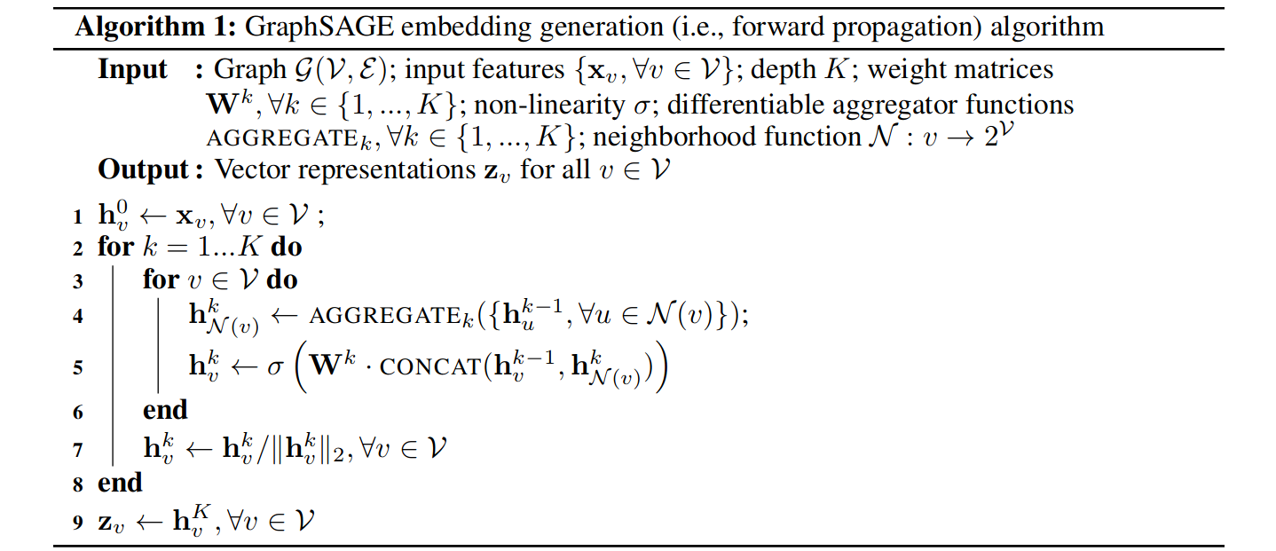
To get the model learning, we need the loss function. For the general unsupervised learning problem, the following loss problem serves pretty well.

This graph-based loss function encourages nearby nodes to have similar representations, while enforcing that the representations of disparate nodes are highly distinct.
For supervised learning, either we can learn the embeddings first and then use those embeddings for the downstream task or combine both the part of learning embeddings and the part of applying these embeddings in the task into a single end to end model and then use the loss for the final part, and backpropagate to learn the embeddings while solving the task simultaneously.
Aggregator Architectures
One of the critical difference between GCN and Graphsage is the generalisation of the aggregation function, which was the mean aggregator in GCN. So rather than only taking the average, we use generalised aggregation function in GraphSAGE.
Mean Aggregator
Mean aggregator is as simple as you thought it would be. Simply take the elementwise mean of the vectors in {huk-1 ∀u ∈ N (v)}. In other words, we can average embeddings of all nodes in the neighbourhood to construct the neighbourhood embedding.

Pool Aggregator
Until now, we were using a weighted average type of approach. But we could also use pooling type of approach; for example, we can do elementwise ‘min’ or ‘max’ pooling. So this would be another option where in we are taking the messages from the neighbours, transforming them and applying some pooling technique ( max-pooling or min pooling ).

In the above equation, ‘max’ denotes the elementwise max operator, and $\sigma$ is a nonlinear activation function (yes you are right it can be ReLU). Please note that the function applied before the max-pooling can be an arbitrarily deep multi-layer perceptron, but in the original paper, simple single-layer architectures is preferred.
LSTM Aggregator
We could also use a deep neural network like Long Short Term Memory RNNs to learn how to aggregate the neighbours. Order invariance is important in the aggregator function, but since LSTM is not order invariant, one would have to train the LSTM over several random orderings or permutation of neighbours to make it invariant of sequence.
Inductive capability
One interesting property of GraphSAGE is that we can train our model on one subset of the graph and apply this model on another subset of this graph. The reason we can do this is that we can do parameter sharing, i.e. those processing boxes are the same everywhere (W and B are shared across all the computational graphs or architectures). So when a new architecture comes into play, we can borrow the parameters (W and B), do a forward pass, and we get our prediction.

This property of GraphSAGE is advantageous in the prediction of protein interaction. For example, we can train our model on protein interaction graph from model organism A (left-hand side in the figure below) and generate embedding on newly collected data from other model organism say B (right-hand side in the figure).
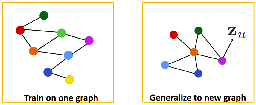
We know that our old methods like DeepWalk were not able to generalise to a new unseen graph. So if any new node gets added to the graph, we had to train our model from scratch, but since our new method is generalised to the unseen graphs, so to predict the embeddings of the new node we have to make the computational graph of the new node, transfer the parameters to the unseen part of the graph and we can make predictions.
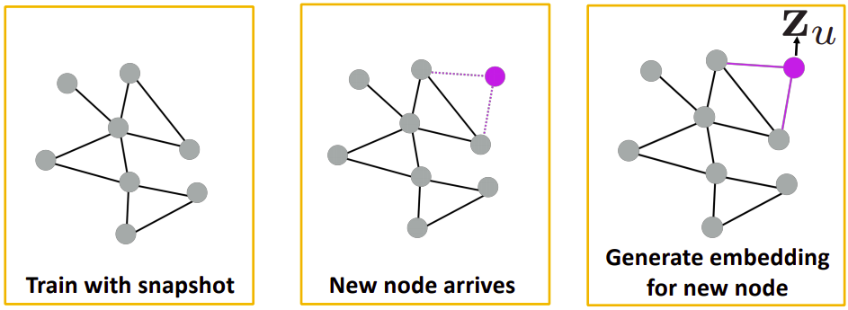
We can use this property in social-networks (like Facebook). Consider the first graph in the above figure, users in a social-network are represented by the nodes of the graph. Initially, we would train our model on this graph. After some time suppose another user is added in the network, now we don’t have to train our model from scratch on the second graph, we will create the computational graph of the new node, borrow the parameters from the already trained model and then we can find the embeddings of the newly added user.
Implementation in PyTorch
|
|
You can find our implementation made using PyTorch in the following GraphSAGE Notebook.
References
-
https://cs.stanford.edu/people/jure/pubs/graphsage-nips17.pdf
-
Graph Node Embedding Algorithms (Stanford - Fall 2019) by Jure Leskovec
Written By
- Ajit Pant
- Shubham Chandel
- Shashank Gupta
- Anirudh Dagar
