The choice of Optimisation Algorithms and Loss Functions for a deep learning model can play a big role in producing optimum and faster results. Before we begin, let us see how different components of a deep learning model affect its result through the simple example of a Perceptron.

Perceptron

If you are not familiar with the term perceptron, it refers to a particular supervised learning model, outlined by Rosenblatt in 1957. The architecture and behavior of a perceptron is very similar to biological neurons, and is often considered as the most basic form of neural network. Other kinds of neural networks were developed after the perceptron, and their diversity and applications continue to grow. It is easier to explain the constitutes of a neural network using the example of a single layer perceptron.

A single layer perceptron works as a linear binary classifier. Consider a feature vector [x1, x2, x3] that is used to predict the probability (p) of occurrence of a certain event.

Weighing factors: Each input in the feature vector is assigned its own relative weight (w), which decides the impact that the particular input needs in the summation function. In relatively easier terms, some inputs are made more important than others by giving them more weight so that they have a greater effect in the summation function (y). A bias (wo) is also added to the summation.

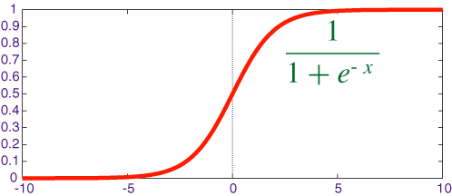
**Activation function: **The result of the summation function, that is the weighted sum, is transformed to a desired output by employing a non linear function (fNL), also known as activation function. Since the desired output is probability of an event in this case, a sigmoid function can be used to restrict the results (y) between 0 and 1.

Other commonly used activation functions are Rectified Linear Unit (ReLU), Tan Hyperbolic (tanh) and Identity function.

**Error and Loss Function: **In most learning networks, error is calculated as the difference between the actual output and the predicted output.

The function that is used to compute this error is known as Loss Function J(.). Different loss functions will give different errors for the same prediction, and thus have a considerable effect on the performance of the model. One of the most widely used loss function is mean square error, which calculates the square of difference between actual value and predicted value. Different loss functions are used to deal with different type of tasks, i.e. regression and classification.

Back Propogation and Optimisation Function: Error J(w) is a function of internal parameters of model i.e weights and bias. For accurate predictions, one needs to minimize the calculated error. In a neural network, this is done using back propagation. The current error is typically propagated backwards to a previous layer, where it is used to modify the weights and bias in such a way that the error is minimized. The weights are modified using a function called Optimization Function.

Optimisation functions usually calculate the gradient i.e. the partial derivative of loss function with respect to weights, and the weights are modified in the opposite direction of the calculated gradient. This cycle is repeated until we reach the minima of loss function.

Thus, the components of a neural network model i.e the activation function, loss function and optimization algorithm play a very important role in efficiently and effectively training a Model and produce accurate results. Different tasks require a different set of such functions to give the most optimum results.

Loss Functions:

Thus, loss functions are helpful to train a neural network. Given an input and a target, they calculate the loss, i.e difference between output and target variable. Loss functions fall under four major category:

**Regressive loss functions: **They are used in case of regressive problems, that is when the target variable is continuous. Most widely used regressive loss function is Mean Square Error. Other loss functions are:

1. Absolute error — measures the mean absolute value of the element-wise difference between input;
2. Smooth Absolute Error — a smooth version of Abs Criterion.

**Classification loss functions: ** The output variable in classification problem is usually a probability value f(x), called the score for the input x. Generally, the magnitude of the score represents the confidence of our prediction. The target variable y, is a binary variable, 1 for true and -1 for false. On an example (x,y), the margin is defined as yf(x). The margin is a measure of how correct we are. Most classification losses mainly aim to maximize the margin. Some classification algorithms are:

1. Binary Cross Entropy
2. Negative Log Likelihood
3. Margin Classifier
4. Soft Margin Classifier

**Embedding loss functions: **It deals with problems where we have to measure whether two inputs are similar or dissimilar. Some examples are:

1. L1 Hinge Error- Calculates the L1 distance between two inputs.
2. Cosine Error- Cosine distance between two inputs.

Visualising Loss Functions:

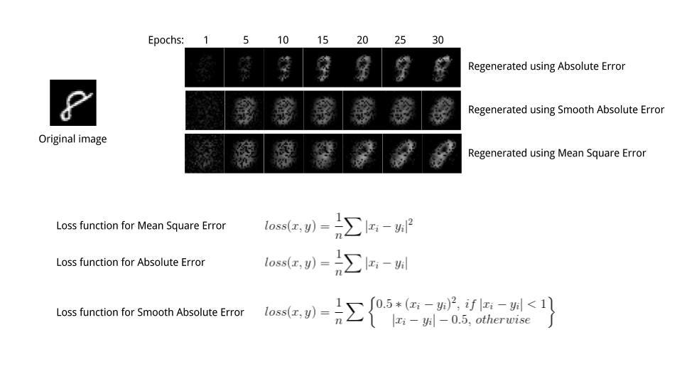
We performed the task to reconstruct an image using a type of neural network called Autoencoders. Different results were obtained for the same task by using different Loss Functions, while everything else in the neural network architecture remained constant. Thus, the difference in result represents the properties of the different loss functions employed. A very simple data set, MNIST data set was used for this purpose. Three loss functions were used to reconstruct images.

1. Absolute Loss Function

2. Mean Square Loss Funtion

3. Smooth Absolute Loss Function.

While the Absolute error just calculated the mean absolute value between of the pixel-wise difference, Mean Square error uses mean squared error. Thus it was more sensitive to outliers and pushed pixel value towards 1 (in our case, white as can be seen in image after first epoch itself).

Smooth L1 error can be thought of as a smooth version of the Absolute error. It uses a squared term if the squared element-wise error falls below 1 and L1 distance otherwise. It is less sensitive to outliers than the Mean Squared Error and in some cases prevents exploding gradients.

Optimisation Algorithms

Optimisation Algoritms are used to update weights and biases i.e. the internal parameters of a model to reduce the error. They can be divided into two categories:

**Constant Learning Rate Algorithms: **Most widely used Optimisation Algorithm, the Stochastic Gradient Descent falls under this category.

Here **η **is called as learning rate which is a hyperparameter that has to be tuned. Choosing a proper learning rate can be difficult. A learning rate that is too small leads to painfully *slow convergence i.e *will result in small baby steps towards finding optimal parameter values which minimize loss and finding that valley which directly affects the overall training time which gets too large. While a learning rate that is too large can hinder convergence and cause the loss function to fluctuate around the minimum or even to diverge.

A similar hyperparameter is momentum, which determines the velocity with which learning rate has to be increased as we approach the minima.

**Adaptive Learning Algorithms: ** The challenge of using gradient descent is that their hyper parameters have to be defined in advance and they depend heavily on the type of model and problem. Another problem is that the same learning rate is applied to all parameter updates. If we have sparse data, we may want to update the parameters in different extent instead.

Adaptive gradient descent algorithms such as Adagrad, Adadelta, RMSprop, Adam, provide an alternative to classical SGD. They have per-paramter learning rate methods, which provide heuristic approach without requiring expensive work in tuning hyperparameters for the learning rate schedule manually.

Working with Optimisation Functions:

We used three first order optimisation functions and studied their effect.

1. Stochastic Gradient Decent

2. Adagrad

3. Adam

**Gradient Descent **calcultes gradient for the whole dataset and updates values in direction opposite to the gradients until we find a local minima. Stochastic Gradient Descent performs a parameter update for each training example unlike normal Gradient Descent which performs only one update. Thus it is much faster. Gradient Decent algorithms can further be improved by tuning important parametes like momentum, learning rate etc.

Adagrad is more preferrable for a sparse data set as it makes big updates for infrequent parameters and small updates for frequent parameters. It uses a different learning Rate for every parameter θ at a time step based on the past gradients which were computed for that parameter. Thus we do not need to manually tune the learning rate.

Adam stands for Adaptive Moment Estimation. It also calculates different learning rate. Adam works well in practice, is faster, and outperforms other techniques.

Stochastic Gradient Decent was much faster than the other algorithms but the results produced were far from optimum. Both, Adagrad and Adam produced better results that SGD, but they were computationally extensive. Adam was slightly faster than Adagrad. Thus, while using a particular optimization function, one has to make a trade off between more computation power and more optimum results.

Torch:

We worked with Torch7 to complete this project, which is a Lua based predecessor of PyTorch.

The github repo of the complete project and codes is- https://github.com/dsgiitr/Visualizing-Loss-Functions

References:

1. https://github.com/torch/nn/blob/master/doc/criterion.md

2. http://christopher5106.github.io/deep/learning/2016/09/16/about-loss-functions-multinomial-logistic-logarithm-cross-entropy-square-errors-euclidian-absolute-frobenius-hinge.html

3. http://news.mit.edu/2015/optimizing-optimization-algorithms-0121

Thanks for reading and keep following our blog series on Deep Learning.