The end is near. No, not the world, but the 12A12D series. After Linear Regression, it’s time to add more DS flavour.

This will teach you a new technique used in case of Overfitting.

I believe this is not the end, but the beginning.

Problem of Overfitting

Occurs when you build a model that not only captures the signal, but also the noise in a dataset. We want to create models that generalise and perform well on different data-points - AVOID Overfitting! In comes Regularization, which is a powerful mathematical tool for reducing overfitting within our model. In this article, I have explained the complex science behind ‘Ridge Regression‘ and ‘Lasso Regression‘ which are the most fundamental regularization techniques, sadly still not used by many.

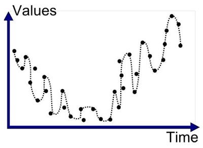
Overfitting or High Variance is caused by a hypothesis function that fits the available data but does not generalise well to predict new data. It is usually caused by a complicated function that creates a lot of unnecessary curves and angles unrelated to the data.

This behaviour of the model is not desired as it has very poor predictive power. There are two main options to address the issue of overfitting:

• Reduce the number of features

• Regularization: When a lot of slightly useful features are there.

What is Regularization?

Linear Regression: The parameters are estimated using the Least Squares approach, where the cost function i.e. the sum of squared residuals (RSS) are minimised.

To perform Regularization, we will be modifying our Cost Function by adding a penalty to RSS. By adding a penalty to the Cost Function, the values of the parameters would decrease and thus the overfitted model gradually starts to smooth out depending on the magnitude of the penalty added.

Ridge Regression

It performs ‘L2 regularization’, i.e. adds penalty equivalent to square of the magnitude of coefficients. Thus, it optimises the following:

_Objective = RSS + α _ (sum of square of coefficients)*

Here, α(alpha) is the tuning parameter which balances the amount of emphasis given to minimising RSS vs minimising sum of square of coefficients. It can take various values:

α = 0:

• The objective becomes same as simple linear regression.

• We’ll get the same coefficients as simple linear regression.

α = ∞:

• The coefficients will be zero. Why? Because of infinite weightage on square of coefficients, anything less than zero will make the objective infinite.

0 < α < ∞:

• The magnitude of α will decide the weightage given to different parts of objective.

• The coefficients will be somewhere between 0 and ones for simple linear regression.

A snippet explaining how to execute Ridge Regression in Python is shown below. For further clarification on the syntax, one can visit Sklearn.

1
2
3
4
5
6
7
8

from sklearn.linear_model import Ridge
import numpy as np
n_samples, n_features = 10, 5
np.random.seed(0)
y = np.random.randn(n_samples)
X = np.random.randn(n_samples, n_features)
clf = Ridge(alpha=1.0)
clf.fit(X, y)

Lasso Regression

LASSO stands for Least Absolute Shrinkage and Selection Operator. I know it doesn’t give much of an idea but there are 2 key words here - absolute and selection.

Lasso regression performs L1 regularization, i.e. it adds a factor of sum of absolute value of coefficients in the optimisation objective.

Objective = RSS + α * (sum of absolute value of coefficients)

Here, α (alpha) works similar to that of ridge. Like that of ridge, α can take various values and provide a trade-off between balancing RSS and magnitude of coefficients.

So till now its *appearing to be very similar to Ridge, *but hold on you’ll know the difference by the time we finish. Like before, snippet follows. For further clarification you can again visit Sklearn.

1
2
3
4
5
6
7

from sklearn import linear_model
clf = linear_model.Lasso(alpha=0.1)
clf.fit([[0,0], [1, 1], [2, 2]], [0, 1, 2])

print(clf.coef_)

print(clf.intercept_)

Selection of α

Alpha can be adjusted to help you find a good fit for your model.

• However, a value that is too low might not do anything.

• One that is too high might actually cause you to under-fit the model and lose valuable information.

It’s up to the user to find the sweet spot. Cross validation using different values of alpha can help you to identify the optimal alpha that produces the lowest out of sample error.

Key differences between Ridge and Lasso Regression

Ridge: It includes all (or none) of the features in the model. Thus, the major advantage of ridge regression is coefficient shrinkage and reducing model complexity.

Lasso: Along with shrinking coefficients, lasso performs feature selection as well. (Remember the ‘selection‘ in the lasso full-form?) As we observed earlier, some of the coefficients become exactly zero, which is equivalent to the particular feature being excluded from the model.

But why is it that the lasso, unlike ridge regression, results in coefficient estimates that are exactly equal to zero? Lets explain it in detail in the next section.

Variable Selection Property of Lasso

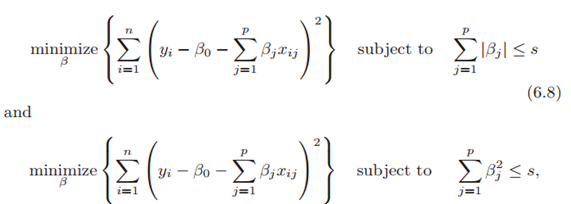
Before explaining this property, let’s look at another way of writing minimisation objective. One can show that the lasso and ridge regression coefficient estimates solve the problems respectively.

In other words, for every value of α, there is some ‘s’ such that the equations (old and new cost functions) will give the same coefficient estimates. When p=2, then (6.8) indicates that the lasso coefficient estimates have the smallest RSS out of all points that lie within the diamond defined by |β1|+ |β2|≤s. Similarly, the ridge regression estimates have the smallest RSS out of all points that lie within the circle defined by (β1)²+(β2)²≤s

Now, the above formulations can be used to shed some light on the issue.

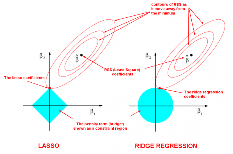
The least squares solution is marked as βˆ, while the blue diamond and circle represent the lasso and ridge regression constraints as explained above. If ‘s’ is sufficiently large, then the constraint regions will contain βˆ, and so the ridge regression and lasso estimates will be the same as the least squares estimates. (Such a large value of s corresponds to α=0 in the original cost function). However, in figure, the least squares estimates lie outside of the diamond and the circle, and so the least squares estimates are not the same as the lasso and ridge regression estimates. The ellipses that are centered around βˆ represent regions of constant RSS.

In other words, all of the points on a given ellipse share a common value of the RSS. As the ellipses expand away from the least squares coefficient estimates, the RSS increases. The above equations indicate that the lasso and ridge regression coefficient estimates are given by the first point at which an ellipse contacts the constraint region.

Since, ridge regression has a circular constraint with no sharp points, this intersection will not generally occur on an axis, and so the ridge regression coefficient estimates will be exclusively non-zero. However, the lasso constraint has corners at each of the axes, and so the ellipse will often intersect the constraint region at an axis. When this occurs, one of the coefficients will equal zero. In higher dimensions, many of the coefficient estimates may equal zero simultaneously. In figure, the intersection occurs at β1=0, and so the resulting model will only include β2.

Applications

• Ridge: In majority of the cases, it is used to prevent overfitting. Since it includes all the features, it is not very useful in case of exorbitantly high features, say in millions, as it will pose computational challenges.

• Lasso: Since it provides sparse solutions, it is generally the model of choice (or some variant of this concept) for modelling cases where the features are in millions or more. In such a case, getting a sparse solution is of great computational advantage as the features with zero coefficients can simply be ignored.

Key Notes

Regularization techniques has its applications everywhere like it has been used in medical sciences to analyse and then study the syphilis data. It was even used for analysis of agricultural economics where the problem of multicollinearity was encountered in past.

Note: While performing regularization techniques, you should standardise your input dataset so that it is distributed according to N(0,1), since solutions to the regularised objective function depend on the scale of your features.

A technique known as Elastic Nets, which is a combination of Lasso and Ridge regression is used to tackle the limitations of both Ridge and Lasso Regression. One can refer to this Link for further details regarding this technique.

References

1. Stanford University slides (For in depth mathematics)

2. Implementation on Kaggle dataset.

3. Scikit Learn documentation.

Footnotes

This was one of the most tech-heavy algorithm in our blog series. I hope that you had a great learning experience. Thanks for supporting us! Here’s all from 12A12D. Till next time, keep learning and improving.

Thanks for reading. :) And, ❤ if this was a good read. Enjoy!

Editor: Akhil Gupta