What are word embeddings? Why we use word embeddings? Before going into details. lets see some example :

1. There are many website that ask us to give reviews or feedback about there product when we are using them. like:- Amazon, IMDB.

2. we also use to search at google with couple of words and get result related to it.

3. There are some sites that put tags on the blog related the material in the blog.

so how do they do this. Actually these things are application of Text processing. we use text to do sentiment analysis, clustering similar word, document classification and tagging.

As we read any newspaper we can say that what is the news about but how computer will do these things? Computer can match strings and can tell us that they are same or not But how do we make computers tell you about football or Ronaldo when you search for Messi?

For tasks like object or speech recognition we know that all the information required to successfully perform the task is encoded in the data (because humans can perform these tasks from the raw data). However, natural language processing systems traditionally treat words as discrete atomic symbols, and therefore ‘cat’ may be represented as Id537 and ‘dog’ as Id143. These encodings are arbitrary, and provide no useful information to the system regarding the relationships that may exist between the individual symbols.

Here comes word embeddings. word embeddings are nothing but numerical representations of texts.

There are many different types of word embeddings:

1. Frequency based embedding

2. Prediction based embedding

Frequency based embedding:

Count vector:

count vector model learns a vocabulary from all of the documents, then models each document by counting the number of times each word appears. For example, consider we have D documents and T is the number of different words in our vocabulary then the size of count vector matrix will be given by D*T . Let’s take the following two sentences:

Document 1: “The cat sat on the hat”

Document 2: “The dog ate the cat and the hat”

From these two documents, our vocabulary is as follows:

{ the, cat, sat, on, hat, dog, ate, and }

so D = 2, T = 8

Now, we count the number of times each word occurs in each document. In Document 1, “the” appears twice, and “cat”, “sat”, “on”, and “hat” each appear once, so the feature vector for documents is:

{ the, cat, sat, on, hat, dog, ate, and }

so the count vector matrix is :-

Now, a column can also be understood as word vector for the corresponding word in the matrix M. For example, the word vector for ‘cat’ in the above matrix is [1,1] and so on.Here, the rows correspond to the documents in the corpus and the columns correspond to the tokens in the dictionary. The second row in the above matrix may be read as — Document 2 contains ‘hat’: once, ‘dog’: once and ‘the’ thrice and so on.

There is a problem related to dimensions of the matrix for a large corpus of text so we can use stop words (remove common words like ‘a, an, this, that’) or we can extract some top words from vocabulary based on frequency and use as a new vocabulary or we can use both methods.

TF-IDF vectorization:

In a large text corpus, some words will be very present (e.g. “the”, “a”, “is” in English) hence carrying very little meaningful information about the actual contents of the document. If we were to feed the direct count data directly to a classifier those very frequent terms would shadow the frequencies of rarer yet more interesting terms.

In order to re-weight the count features into floating point values suitable for usage by a classifier it is very common to use the tf–idf transform. This method takes into account not just the occurrence of a word in a single document but in the entire corpus. lets take a business article this article will contain more business related terms like Stock-market, Prices, shares etc in comparison to any other article. but terms like “a, an, the” will come in each article with high frequency. so this method will penalize these type of high frequency words.

Tf means term-frequency while tf–idf means term-frequency times inverse document-frequency.

TF = (Number of times term t appears in a document)/(Number of terms in the document)

IDF = log(N/n), where, N is the total number of documents and n is the number of documents a term t has appeared in.

TF-IDF(t, document) = TF(t, document) * IDF(t)

Co-Occurrence Matrix with a fixed context window

Words co-occurrence matrix describes how words occur together that in turn captures the relationships between words. Words co-occurrence matrix is computed simply by counting how two or more words occur together in a given corpus. As an example of words co-occurrence, consider a corpus consisting of the following documents:

penny wise and pound foolish

a penny saved is a penny earned

Letting count(w(next)|w(current)) represent how many times word *w(next) *follows the word w(current), we can summarize co-occurrence statistics for words “a” and “penny” as:

The above table shows that “a” is followed twice by “penny” while words “earned”, “saved”, and “wise” each follows “penny” once in our corpus. Thus, “earned” is one out of three times probable to appear after “penny.” The count shown above is called bigram frequency; it looks into only the next word from a current word. Given a corpus of N words, we need a table of size NxN to represent bigram frequencies of all possible word-pairs. Such a table is highly sparse as most frequencies are equal to zero. In practice, the co-occurrence counts are converted to probabilities. This results in row entries for each row adding up to one in the co-occurrence matrix.

But, remember this co-occurrence matrix is not the word vector representation that is generally used. Instead, this Co-occurrence matrix is decomposed using techniques like PCA, SVD etc. into factors and combination of these factors forms the word vector representation.

Let me illustrate this more clearly. For example, you perform PCA on the above matrix of size NXN. You will obtain V principal components. You can choose k components out of these V components. So, the new matrix will be of the form N X k.

And, a single word, instead of being represented in N dimensions will be represented in k dimensions while still capturing almost the same semantic meaning. k is generally of the order of hundreds.

So, what PCA does at the back is decompose Co-Occurrence matrix into three matrices, U,S and V where U and V are both orthogonal matrices. What is of importance is that dot product of U and S gives the word vector representation and V gives the word context representation.

Advantages of Co-occurrence Matrix

1. It preserves the semantic relationship between words. i.e man and woman tend to be closer than man and apple.

2. It uses SVD at its core, which produces more accurate word vector representations than existing methods.

3. It uses factorization which is a well-defined problem and can be efficiently solved.

4. It has to be computed once and can be used anytime once computed. In this sense, it is faster in comparison to others.

Disadvantages of Co-Occurrence Matrix

1. It requires huge memory to store the co-occurrence matrix. But, this problem can be circumvented by factorizing the matrix out of the system for example in Hadoop clusters etc. and can be saved.

Applications of frequency based methods:

The frequency based methods are easy to understand and their are many applications of them like text classification, sentiment analysis and many more. Because they extract positive and negative words from the text so we can easily classify them with the help of any good machine learning algorithms.

Prediction based methods:

Continuous Bag of Words(CBOW):

CBOW is learning to predict the word by the context. A context may be single word or multiple word for a given target words.

lets see this by an example “The cat jumped over the puddle.”

So one approach is to treat {“The”, “cat”, ’over”, “the’, “puddle”} as a context and from these words, be able to predict or generate the center word “jumped”. This type of model we call a Continuous Bag of Words (CBOW) Model.

**Before going in detail in CBOW lets talk about one hot representation of words : **One way to represent a word as a vector is one-hot representation. One-hot representation is a representation method in which only one element is 1 and the other elements are 0 in the vector. By setting 1 or 0 for each dimension, it represents “that word or not”.

Let’s say, for example, we represent the word “python” as one-hot representation. Here, the vocabulary which is a set of words is five words(nlp, python, word, ruby, one-hot). Then the following vector expresses the word “python”:

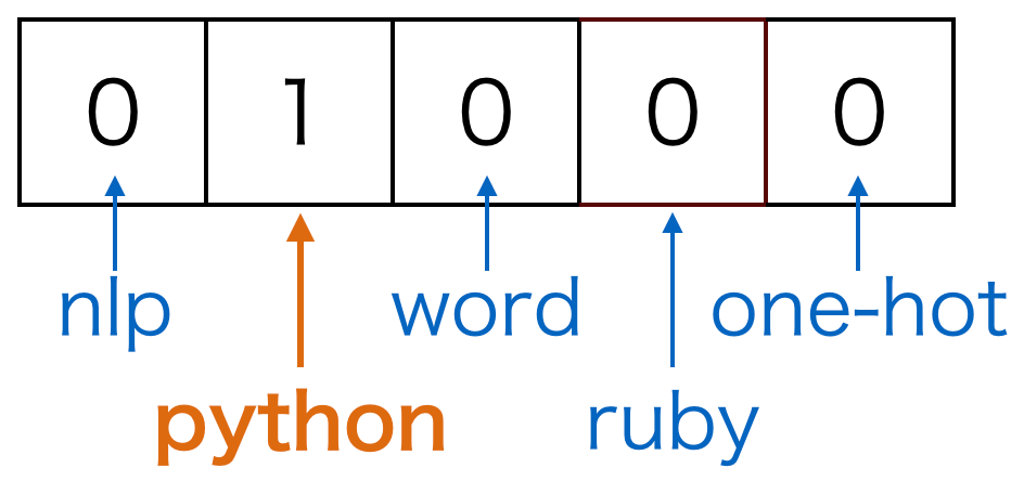
Although one-hot representation is simple, there are weak points: it is impossible to obtain meaningful results with arithmetic between vectors. Let’s say we take an inner product to calculate similarity between words. In one-hot representation, different words are 1 in different places and the other elements are 0. Thus, the result of taking the dot product between the different words is 0. This is not a useful result.

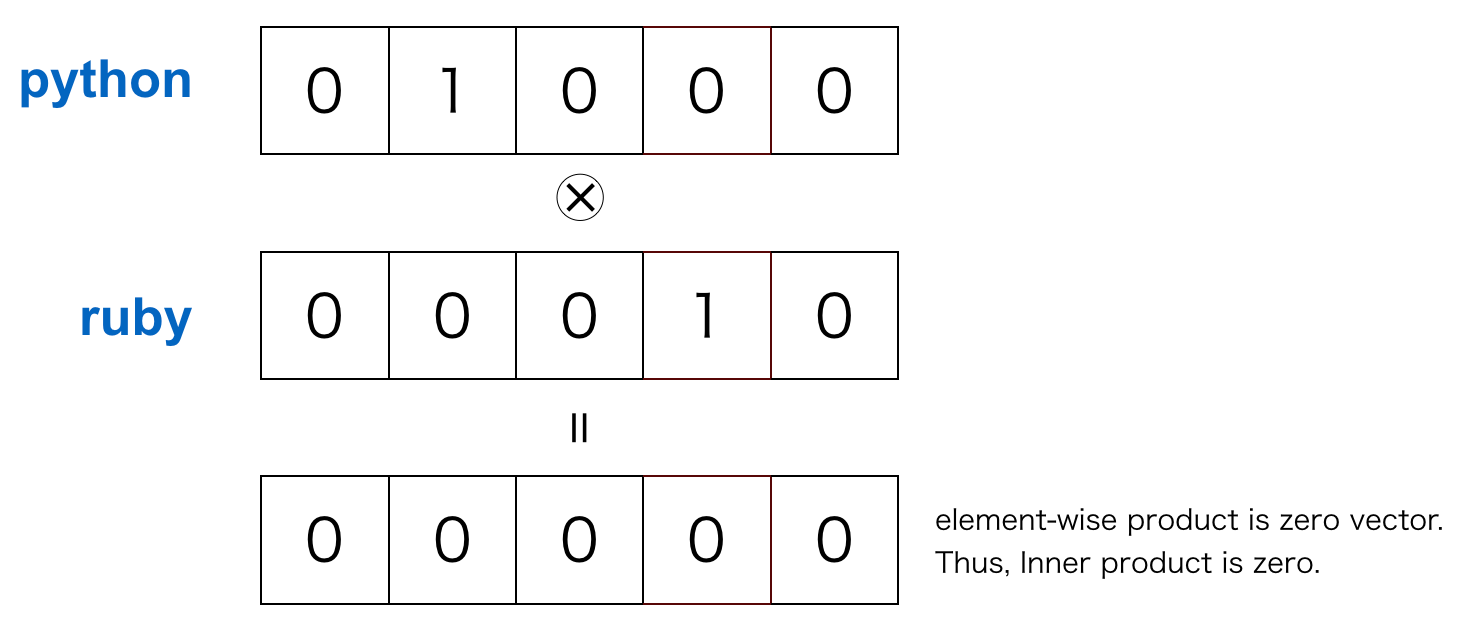
Another weak point is the vector tend to become very high dimension. Since one dimension is assigned to one word, as the number of vocabularies increases, it becomes very high dimension.

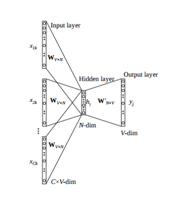
We breakdown the way this model works in these steps:

Wi = weight matrix between input layer and hidden layer of size [V * N]

Wj= weight matrix between hidden layer and output layer of size [N * V]

1. We generate our one hot word vectors (x (c−m) , . . . , x (c−1) , x (c+1) , . . . , x (c+m) ) for the input context of size m. where x(c) is the center or target word that we want to predict. we have C(= 2m) one hot word vector of size [1 * V]. so our input layer size is [C * V]

2. We than multiply them with matrix Wi to get our embedded words of size [1 * N].

3. Now we take average of these 2m [1 * N] vectors.

4. Now we calculate the hidden layer output by multiplying hidden layer input with matrix Wj. Now we get a score vector of size[1 * V]. lets name it z.

5. Turn the scores into probabilities by yˆ = softmax(z)

6. We desire our probabilities generated, yˆ, to match the true probabilities, y, which also happens to be the one hot vector of the actual word.

7. Error between output and target is calculated and propagated back to re-adjust the weights.

The loss function used is Cross entropy.

and then we use gradient descent or any good optimizer to train this network. After training the weight between the hidden layer and the output layer (Wj) is taken as the word vector representation of the word. where each column represent a word vector of size [1 * N].

Skip-gram model:

Another approach is to create a model such that given the center word “jumped”, the model will be able to predict or generate the surrounding words “The”, “cat”, “over”, “the”, “puddle”. Here we call the word “jumped” the context. We call this type of model a SkipGram model.

Skip-gram model reverses the use of target and context words. Skip-gram take a word and predict the context word from it.

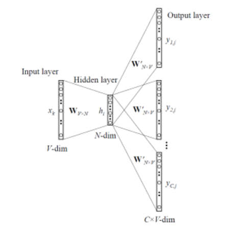
We breakdown the way this model works in these steps:

Wi = weight matrix between input layer and hidden layer of size [V * N]

Wj= weight matrix between hidden layer and output layer of size [N * V]

1. We generate our one hot word vectors x(c) for the input center word. where (x (c−m) , . . . , x (c−1) , x (c+1) , . . . , x (c+m) ) is the context words that we want to predict. so our input layer size is [1 * V]

2. We than multiply them with matrix Wi to get our embedded words of size [1 * N].

3. Now we calculate the hidden layer output by multiplying hidden layer input with matrix Wj. Now we get C(= 2m) score vector of size[1 * V]. lets name it z(i).

4. Turn the scores into probabilities by yˆ(i) = softmax(z(i))

5. We desire our probabilities generated, yˆ(i), to match the true probabilities, y(i), which also happens to be the one hot vector of the actual words.

6. Error between output and target is calculated and propagated back to re-adjust the weights.

One can ask that all the yˆ are same so how will they help?

yeah, yˆ are all same but their target vectors are different so they all give different error vectors and Element-wise sum is taken over all the error vectors to obtain a final error vector. after that we use the back-propagation algorithm and gradient descent to learn the model.

Advantages/Disadvantages of CBOW and Skip-gram:

1. Being probabilistic is nature, these are supposed to perform superior to deterministic methods(generally).

2. These are low on memory. They don’t need to have huge RAM requirements like that of co-occurrence matrix where it needs to store three huge matrices.

3. Though CBOW (predict target from context) and skip-gram (predict context words from target) are just inverted methods to each other, they each have their advantages/disadvantage. Since CBOW can use many context words to predict the 1 target word, it can essentially **smooth out **over the distribution. This is essentially like regularization and is offer very good performance when our input data is not so large. However the skip-gram model is more fine grained so we are able to extract more information and essentially have more accurate embeddings when we have a large data set (large data is always the best regularizer). Skip-gram with negative sub-sampling outperforms every other method generally.

Application of word embedding(Word2Vec):

There are various NLP based tasks where these word embeddings used in deep learning have surpassed older ML based models. There are various NLP applications where they are used extensively. Eg. Automatic summarization, Machine translation, Named entity resolution, Sentiment analysis, Chat-bot, Information retrieval, Speech recognition, Question answering etc.

We can visualize the learned vectors by projecting them down to 2 dimensions using for instance something like the t-SNE dimensionality reduction technique. When we inspect these visualizations it becomes apparent that the vectors capture some general, and in fact quite useful, semantic information about words and their relationships to one another. It was very interesting when we first discovered that certain directions in the induced vector space specialize towards certain semantic relationships, e.g. male-female, verb tense and even *country-capital *relationships between words, as illustrated in the figure below .

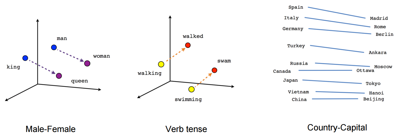
This explains why these vectors are also useful as features for many canonical NLP prediction tasks, such as part-of-speech tagging or named entity recognition.

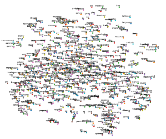
As we can see all the similar words are in together. We can perform some amazing tasks from word embeddings of Word2Vec.

1. Finding the degree of similarity between two words. model.similarity('woman','man') 0.73723527

2. Finding odd one out. model.doesnt_match('breakfast cereal dinner lunch';.split()) 'cereal'

3. Amazing things like woman+king-man =queen model.most_similar(positive=['woman','king'],negative=['man'],topn=1) queen: 0.508

4. Probability of a text under the model model.score(['The fox jumped over the lazy dog'.split()]) 0.21

Word Embeddings is an active research area trying to figure out better word representations than the existing ones. But, with time they have grown large in number and more complex. This article was aimed at simplying some of the workings of these embedding models without carrying the mathematical overhead.

References

1. **Bag of words(count vector) and Word2Vec **Github repository of **DSG.

2. Tf–idf term weighting

3. Co-occurrence matrix with fixed context size

4. [Word2Vec Tutorial (CBOW)](http://mccormickml.com/assets/word2vec/Alex_Minnaar_Word2Vec_Tutorial_Part_II_The_Continuous_Bag-of-Words_Model.pdf)

5. Word2Vec Tutorial (Skip-gram)

6. Word2Vec python implementation

7. [Word2Vec Maths](http://word2vec Parameter Learning Explained)

Footnotes:

One suggestion is that do not miss out references, by reading them only you can understand algorithm properly.

Hit ❤ if this makes you little bit more intelligent.