
This is the winning code for “Eye In The Sky” Satellite Image Segmentation Competetion as a part of Inter-IIT Tech Meet 2018 hosted by IIT Bombay.
Problem Statement
We were provided with a satellite imagery dataset for semantic segmentation and the task was to propose and implement a satellite dense image classification technique.
What exactly is semantic segmentation?
Semantic segmentation for images can be defined as the process of partitioning and classifying the image into meaningful parts, and classify each part at the pixel level into one of the pre-defined classes. The current success of deep learning techniques in computer vision tasks motivated researchers to explore such techniques for pixel-level classification tasks as semantic segmentation.
Motivation
Following the wave of success of Deep learning in various fields and thanks to the increased availability of data and computational resources, the use of deep learning in remote sensing is finally taking off in remote sensing as well. Remote sensing data bring some new challenges for deep learning since satellite image analysis raises some unique questions that translate into challenging new questions:
● Remote sensing data are often multi-modal, e.g. from IR sensors, where both the imaging geometries and the content are completely different. Already prior to a joint information extraction, a crucial step is to develop novel architectures for the matching of images taken from different perspectives and even different imaging modality, preferably without requiring manual inputs.
● Remote sensing data are geo-located, i.e., they are naturally located in the geographical space. Each pixel corresponds to a spatial coordinate, which facilitates the fusion of pixel information with other sources of data. Handling such high dimensional complex data requires automatic extraction and learning of features from satellite images.
Satellite imagery is a rich and structured source of information, yet it is less investigated than everyday images by computer vision researchers. However, automatic segmentation of satellite images could have a critical impact on the way we understand and track the health of our environment and lead to major breakthroughs in global urban planning or climate change research. Traditionally, indexes like Normalized difference vegetation index(NDVI) and Normalized difference water index(NDWI) were used to segment specific classes like water and vegetation using the properties of IR channel in panchromatic images but these methods have very limited success and have a very high false positive rate. Deep learning opens the pathway to a robust and scalable solution for the problem of image segmentation in satellite images.
Classification Approach
Dataset/ Data Analysis
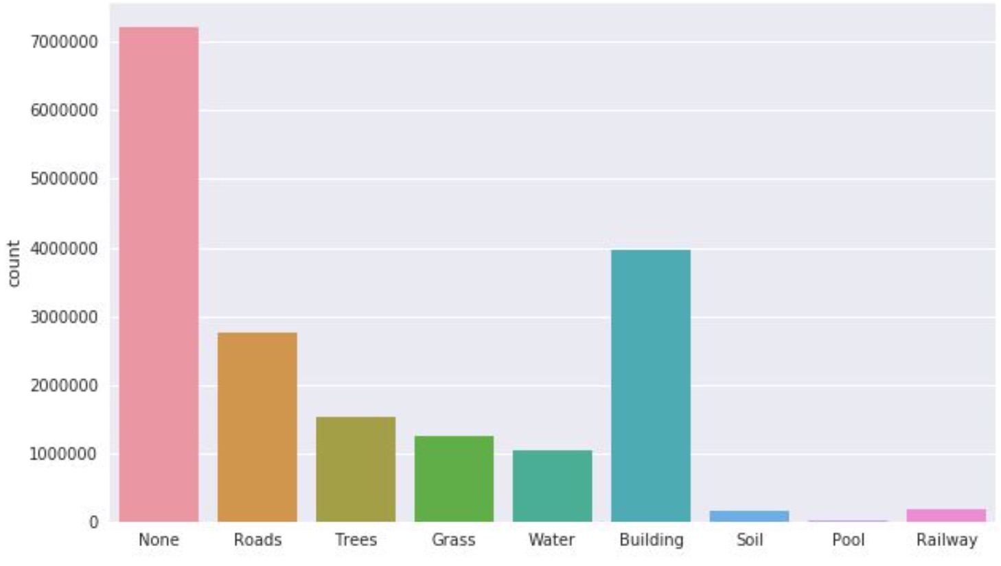
The dataset contained 16 training images and 6 images were given as test data. Images were of varying resolution and contained Near InfraRed channel (NIR) along with regular RGB channels. Images given were saved in uint16 format. There are 8 different classes present in the data along with one none class. We observed the dataset is highly imbalanced as well as skewed in terms of the range of pixel values. We select three images as the validation set in all our experiments such that our validation has balanced class distribution. Images used for validation are 13.tif, 3.tif, 9.tif.
Methodology
We decided to work on two different methods
- Binary image segmentation and recombining(one vs all)
- Multiclass segmentation (all vs all)
Preprocessing
We normalized the input to the networks by subtracting channel wise mean and dividing by channel by variance of the whole training data. We divided the dataset into two parts with thirteen images used for training and three for validation. We created patches with a stride less than the patch size in both directions which led to some overlap to exist between any two consecutive patches. This helped us increase the small training data. As images pixel values were highly skewed we also range normalized the range of the pixels.
Data Augmentation
Generally a large amount of data is required to train a network but in this case, only 16 images were available thus data augmentation plays a very important role. In order to maintain a reasonable amount of images, and above all to avoid overfitting by ensuring a sufficient invariance and robustness of the network, we applied real-time data augmentation techniques to our training set. We used some standard augmentation techniques like horizontal and vertical flip all training images. We also rotated the images by (+20,-20) randomly with a probability of 0.5. During rotation, some new pixel values will be introduced we filled them with a mirror image of the original image data.
Binary Image Segmentation
We trained 8 different binary models on all the classes and then combined all the eight outputs to form the final multiclass segmentation. As it is easier to learn just one class than learning all classes together.
Methods
Model architecture
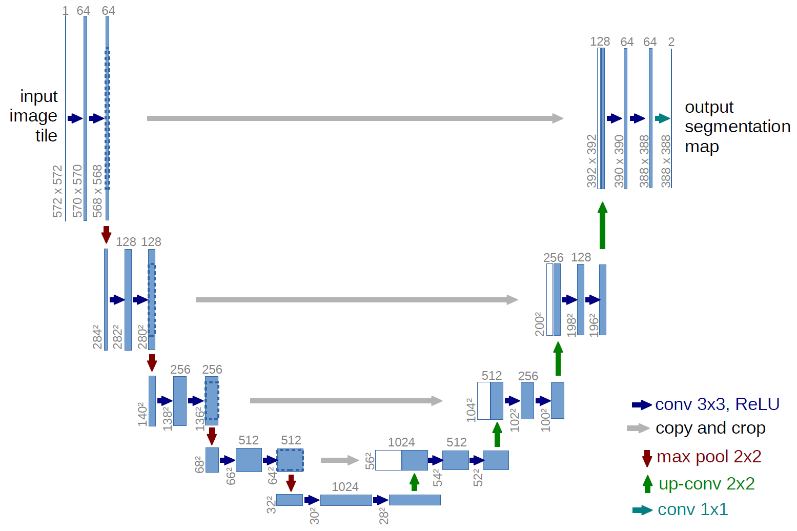
We used encoder-decoder like Fully Convolutional Network inspired from Unet family of networks. Unet was originally developed for biomedical image segmentation.
Why U-Net?
In our case, using a U-Net is a good choice because of the lack of training data, and it also seems to be the choice of most researchers in other fields where image segmentation plays a major role. This neural network architecture has revealed to be very good in this situation. U-Nets have the ability to learn in environments of low to medium quantities of training data, and the amount of training data available in the problem statement is considered low. Also, a U-Net can be very easily adapted to recent research for tweaking the model according to the application.
U-net builds upon Fully Convolutional Network. An encoder extracts features of different levels using convolutions, ReLu activations, and Max pooling. A symmetric encoder path then upsamples the result to increase the resolution of the detected features, skip-connections (concatenations) are added between the contracting path and the expanding path, allowing precise localization as well as context. The expanding path, therefore, consists of a sequence of up-convolutions and concatenations with the corresponding feature map from the contracting path, followed by ReLU activations.
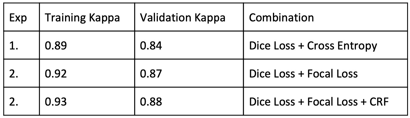
We trained 1 model for each class. Six of them were basic Unets with slight modifications while two used for Road and Railway used Link-Net like architecture. The “Road” class was trained using LinkNet like architecture, with a ResNet34 as its encoder and an Unet like Decoder. We used Dilated Convolutions to incorporate global context in case of road detection. We used Adam optimizer instead of stochastic gradient descent as it is known to converge faster. We also modified the padding to “same” to avoid shrinking during convolution, added Batch Normalization after each ReLU activation to speed up training. We used different loss strategy for different classes which are summarised below in the form of a table.
We used different losses for the different set of classes. We started with Soft Dice Loss but we soon observed that the although dice loss could optimize the overlap the model do not predict sharp images and overall accuracy was still low. To increase the accuracy and sharpness we decided to use Binary cross entropy along with Soft Dice Loss. We used a combination of these losses as well as some variations were made to these loss function to best suit the class.
The loss functions and architectures used are summarised in the table given below:
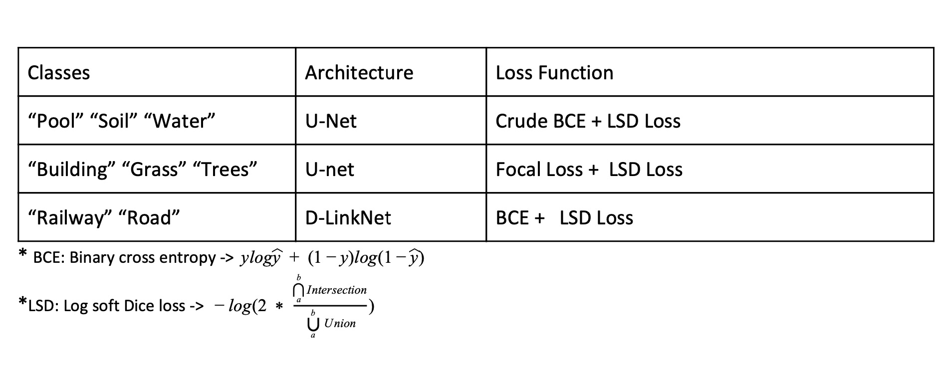
We introduced a novel variant of BCE loss Crude BCE, Which penalizes model predictions based on the expected probability of that class in the mini batch. This Highly reduced the chances of our model predicting some random class at some very unexpected location.

Model Training
Due to the memory constraints available on GPU, we did training in mini-batches of 16. We started with a learning rate of 1e-3 for 20-30 epochs and then fine-tuned the network for 5-10 more epochs with learning rate reduced to one-tenth of its previous value for proper convergence of network. Due to the class imbalance in the dataset, the classes with low representation like “pool”, “Soil”, “Railway”, One of the major problem encountered in Binary segmentation is the absence of positive class. We used patch sampling in data loader with weights assigned to each patch according to the class distribution of the patch. Final weights were calculated as the inverse frequency of a particular class in the training data. Since, classes like Pool and Soil were present in very less amount in training data as compared to other major classes like Building, Grass and None we suspected our model would not generalize very well on these classes. During training, we occasionally observed spurious predictions of these classes in unexpected places. Therefore, to counter this major problem we came up with a novel variant of binary cross entropy loss function namely crude BCE which is described above in the loss function section. We also observed that the binary model trained on water class was confusing with the shadows of buildings.
We suspected the cause of the problem to be IR channel as the Infrared signature of both water and shadows are quite similar.
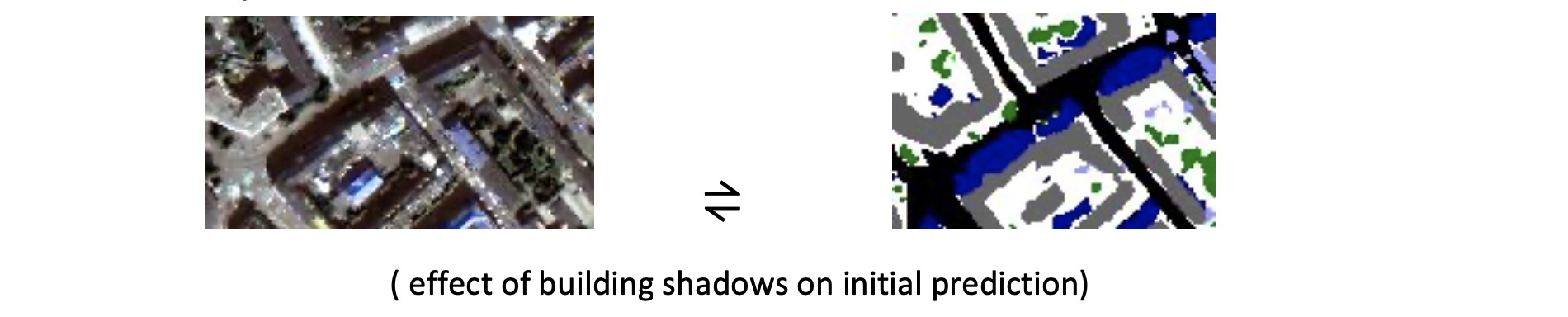
It is to be noted that water class is generally present as a large water body and therefore we penalize our model through crude BCE for small spurious predictions. We also used a simple morphological operation like erosion to remove very small patches of water.
Multi-class Image segmentation
In this methodology, we trained a single Multi-Class Segmentation Model for all the classes except none. Why Multi class? After extensive experimentation on Binary models, we noticed that the final combined predictions from binary models were mainly confused with ‘None’ class which is supported by our confusion matrix presented in the case of binary predictions. One of the reasons behind this is the absence of global context available to the binary models for eg. our fully convolutional models when trained on binary can only learn features specific to the class on which it is trained and lacks the ability to learn the combined features of some closely related classes like Buildings are mostly separated by Roads. Another reason for the same is the presence of a few incorrect annotations in the ground truth data. The ‘None’ class provided in the ground truth in most of the cases doesn’t correspond to a separate class and hence misleads the model at the boundaries of other classes. Unet with ResBlocks This architecture is similar to Unet however the building blocks of the encoder are inspired by ResNet Architecture.The ResBlock consists of Conv ->Relu->BatchNorm->Conv->Relu->BatchNorm.
Why Unet with ResBlocks?
● When deeper Unet is able to start converging, a degradation problem has been exposed: with the network depth increasing, accuracy gets saturated (which might be unsurprising) and then degrades rapidly. Unexpectedly, such degradation is not caused by overfitting and adding more layers to a suitably another deep model which leads to higher training error. It happens due to the fact that deeper networks are harder to optimize. ResBlocks address the degradation problem by introducing a deep residual learning framework.
Loss Functions :
Our Models was optimized for the combination of dice Loss, Cross Entropy and Focal Loss .
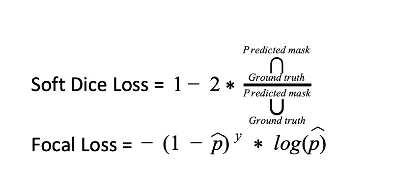
The main aim of dice loss is the optimization of intersection over union and can be used where we cannot guarantee equal distribution of classes.

The Dice Loss optimized the Intersection over Union however, small wrong predictions are not penalized because they have small intersection as compared to the union. So to counter that we also used the Focal Loss which was more focused on the per-pixel predictions. The focal loss was also more focused on the per-pixel loss optimizing the boundaries and can be used where we cannot guarantee equal distribution of classes.
Training:
Training multi-class model is quite similar to the binary case except for the output of the model and ground truth are converted to multi-channel one-hot encoded mask, each channel belongs to one class. Multichannel probability maps are produced as output by using softmax the end of Unet where each channel belongs the confidence score assigned to each class by the model. Training patches of 256x256x4 and a relatively bigger batch size of 16 is used for removing noise in the training We used the same specs as mentioned in the binary case like the use of Adam optimizer. In the case of multi-class models due to the abundance of data belonging to a particular class the need for class balancing is less relatively. Here also we ensured that the underrepresented classes were oversampled through effective augmentations described above in augmentations section. Initially, we trained multi-class model considering the loss on ‘none’ class but later due to the decision of exclusion of ‘none’ class from the evaluation of final metrics we decided not to calculate the loss on ‘none’ channel in output mask and hence made the model ignore ‘none’ class entirely. We used Binary cross entropy and Soft dice loss for final training of network. We also tried experimenting with class weights and sampler in data loader as described in the binary case but we noticed that it didn’t affect the validation metrics much and hence to minimize the computational cost of computing dynamic weights at each training iteration we decided to drop this idea. In multi-class segmentation we noticed that the validation accuracy saturates pretty quickly. We suspected hard negatives as the major reason behind the problem and hence we decided to fine-tune our model for 5-10 epoch with the focal loss which penalizes the model more on hard examples. We tuned the gamma for focal loss and decided gamma=1 as its final value.
Implementation
We used Python programming language and Pytorch framework for coding our deep learning models. The code structure is described in detail in the README.md provided by us in the code folder. We used some important packages like ImgAug for augmentation and Pydencrf for post-processing.
Post processing
We noticed that the U-net sometimes predict coarse segmentation maps. Hence, to counter this we applied test time augmentation belonging to Dihedral group . We predict on four variants of the same patch generated from four-ninety degree rotations. The four probability maps thus generated are rotated back to the original orientation of the image and averaged. The final probability patch for the image is constructed by combining all the patch probability map using bilinear interpolation. The probability map is then finally converted to its RGB counterpart by taking argmax a long the channel dimension. We also tried fully connected conditional random fields as the final post-processing step in order to make our predictions smoother and find a negligible increase in the final validation metric.
Conclusion
In this report, we analyzed the provided dataset and explained our approaches for effective segmentation of satellite images. We experimented extensively and found reasons for the problems being faced in the analysis of the dataset. We also provided the solution to many common problems one can face image segmentation. In conclusion, we would like to add that a successful approach to above-mentioned problems allows to significantly improve the quality of final models. Our approach includes several steps, such as the adaptation of fully convolutional network to multispectral satellite images with joint training objective, handling class imbalance in images and analysis of boundary effects, reflectance indices.
Results
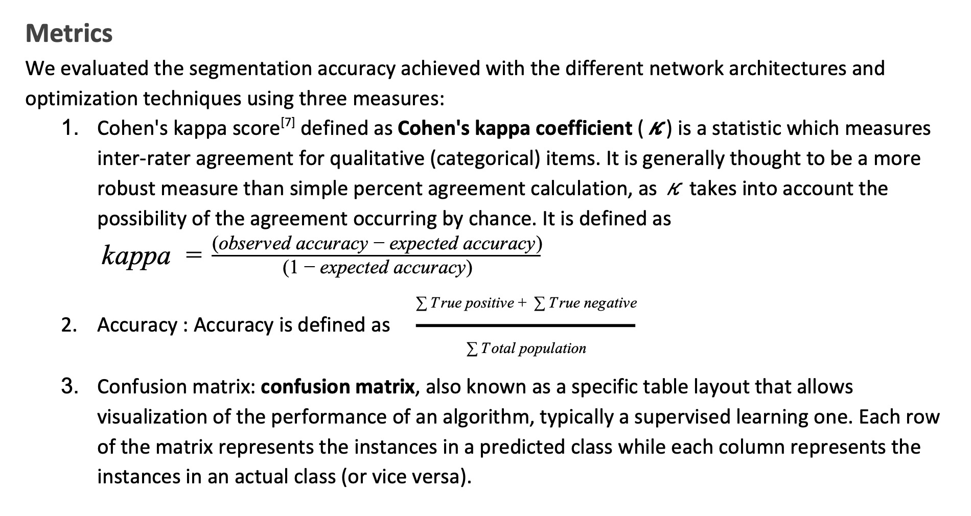
Kappa Score:-
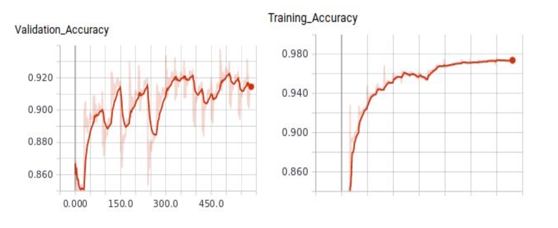
Accuracy:- We achieved a training accuracy of 0.976 and a validation accuracy of 0.920
Confusion Matrix:-
Here classes are numbered from 0 to 7 for classes Roads, Trees, Grass, Building, Soil, Pool, Water and Railways
