Visualising different loss and optimisation functions using Autoencoder.
The aim of the project was to reconstruct images with the help of Autoencoders to visualise the difference in output when different loss or optimisation functions are used. A very simple dataset, MNIST dataset was used for this purpose.
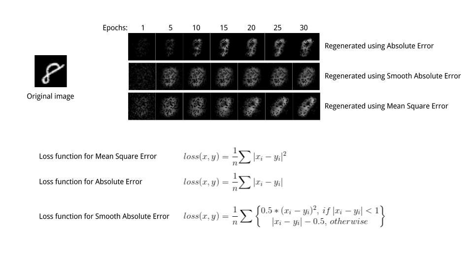
While training a neural network, gradient is calculated according to a given loss function. I compared the results of three regression criterion functions.
- Absolute criterion
- Mean Square Error criterion
- Smooth L1 criterion
While the Absolute error just calculated the mean absolute value between of the pixel-wise difference, Mean Square error uses mean squared error. Thus it is more sensitive to outliers and pushes pixel value towards 1 (in our case, white as can be seen in image after first epoch itself)
Smooth L1 error can be thought of as a smooth version of the Absolute error. It uses a squared term if the squared element-wise error falls below 1 and L1 distance otherwise. It is less sensitive to outliers than the Mean Squared Error and in some cases prevents exploding gradients.
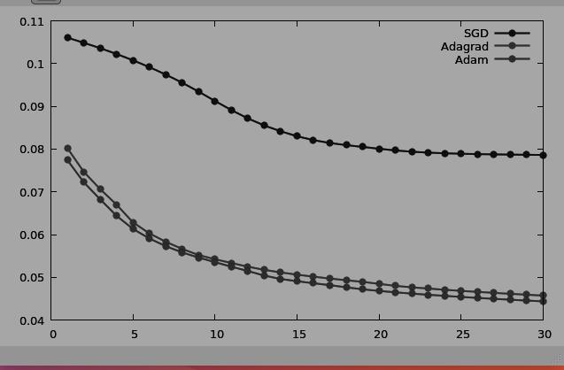
Optimization algorithms helps us to minimize the Loss functions by updating Weights and Biases and reach to the global minima. Some algorithms give faster and slightly better results based on the dataset. We used three first order optimisation functions:
- Stochastic Gradient Decent
- Adagrad
- Adam
Gradient Descent calcultes gradient for the whole dataset and updates values in direction opposite to the gradients until we find a local minima. Stochastic Gradient Descent performs a parameter update for each training example unlike normal Gradient Descent which performs only one update. Thus it is much faster. Gradient Decent algorithms can further be improved by tuning important parametes like momentum, learning rate etc.
Adagrad is more preferrable for a sparse data set as it makes big updates for infrequent parameters and small updates for frequent parameters. It uses a different learning Rate for every parameter θ at a time step based on the past gradients which were computed for that parameter. Thus we do not need to manually tune the learning rate.
Adam stands for Adaptive Moment Estimation. It also calculates different learning rate. Adam works well in practice, is faster, and outperforms other techniques.