Boosting Decrypted
 I know it’s getting arduous to catch up with out daily posts, but it’s just meant to be this. 12 Algos in 12 days. Here, we unbox one of the most powerful ML technique used by Grandmasters to win Data Hackathons on Kaggle. You’ll consider yourself lucky if you understand this properly.
Improving a model accuracy beyond a certain limit can be challenging. This is exactly why you need Boosting.
Don’t give up at half time. Concentrate on winning the second half.
What is Boosting?
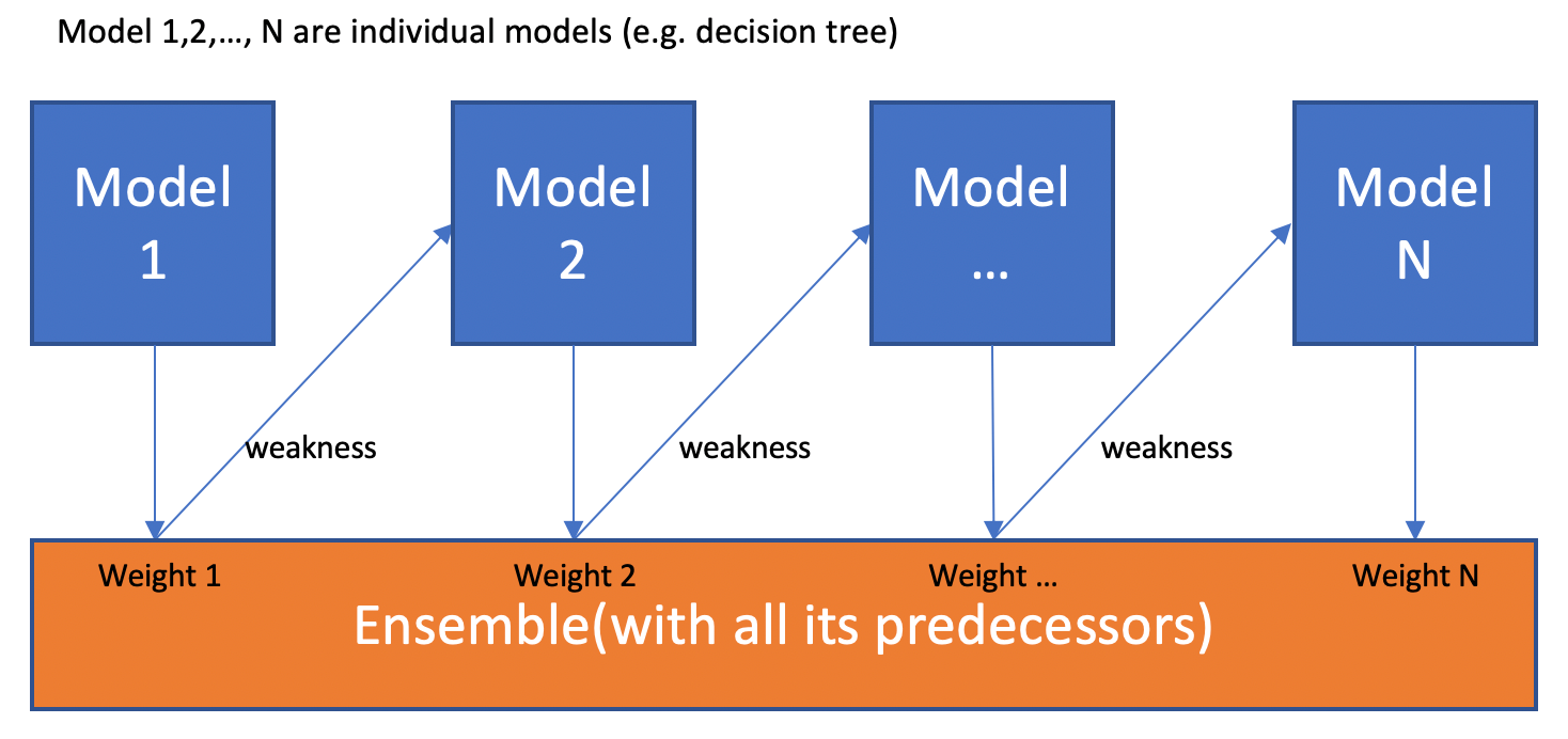
A family of machine learning ensemble meta-algorithms in supervised learning that improve the accuracy of ML algorithms.
Can a set of weak learners create a single strong learner?
Weak learner: Any ML algorithm that provides an accuracy slightly better than random guessing.
Ensemble: The overall model built by Boosting is a weighted sum of all of the weak learners. Overall model yields a pretty high accuracy.
Meta-algorithm: It isn’t a machine learning algorithm itself, uses other algorithms to make stronger predictions.
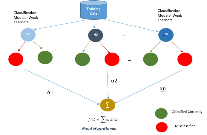
Types of Boosting
1. AdaBoost
First original boosting technique: highly accurate prediction rule by combining many weak and inaccurate rules. Classic use case: Face Detection
Algo explained!
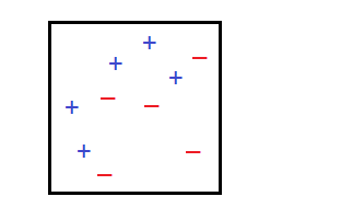
Above shown is the sample space we shall use for classification.
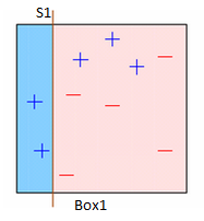
Box1 : Equal weights are assigned to all observations and a decision stump is applied to classify + or - . S1 has generated a vertical line on the left side to classify the data points. This decision stump incorrectly predicted three +. So, we’ll assign more weight to these three data points in our next decision stump.
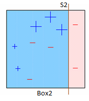
Box2 : The size difference between those three incorrectly predicted and the rest of the data points is clearly visible. Another decision stump (S2) is applied to predict them correctly on the right side of the box. But, this time three - are classified incorrectly. Repeat.
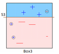
Box3 : Here, three - are given higher weights. S3 is applied to predict these misclassified observations correctly. This time, a horizontal line is generated to classify - and +.
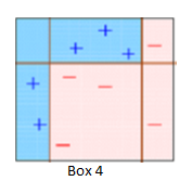
Box4 : Here, we combine S1, S2, and S3 to form a strong prediction having a complex rule as compared to the individual weak learners. Evidently, this algorithm has classified these observations accurately as compared to any of the individual weak learners.
Mostly, we use decision stumps with AdaBoost. But, any machine learning algorithm can be used as base learner if it accepts weights on the training data set. (Both Classification and Regression)
If you are going through hell, keep going. (W. Churchill)
Most Important Parameters
Here, the essential params are explained. Rest can be mugged from Sklearn.
base_estimator: Base estimator from which boosted ensemble is built. Like in given example we used Decision Tree as base learner.
n_estimators: The maximum number of estimators at which boosting is terminated. In case of perfect fit, the learning procedure is stopped early.
learning_rate: Shrinks the contribution of each tree by learning_rate. There is a trade-off between learning_rate and n_estimators.
algorithm: The SAMME.R algorithm typically converges faster than SAMME, achieving a lower test error with fewer boosting iterations.

2. Gradient Boosting
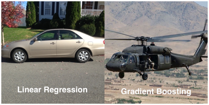
If linear regression was a Toyota Camry, then gradient boosting would be a UH-60 Blackhawk Helicopter. It is the go-to algorithm for most of the hackers aiming to win ML competitions. Read carefully!
ML technique used for regression and classification problems, it produces a prediction model in the form of an ensemble of weak prediction models, typically decision trees. The principle idea behind this algorithm is to construct new base learners which can be maximally correlated with negative gradient of the loss function, associated with the whole ensemble.
Maths Maths and More Maths:
Lets consider a regression problem this time. We are given (x1, y1), (x2, y2), … ,(xn, yn), and the task is to fit a model F(x) to minimize the square loss. Suppose we have a model and the model is good but not perfect. There are some mistakes: F(x1) = 0.8, while y1 = 0.9, and F(x2) = 1.4 while y2 = 1.3… How can we improve this model without remove anything from F or change in any parameter of F?
We can add an additional model (regression tree) h to F, so that the new prediction will be F(x) + h(x).
we wish to improve the model such that
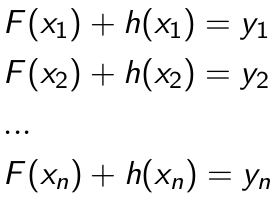
Or, equivalently, you wish that
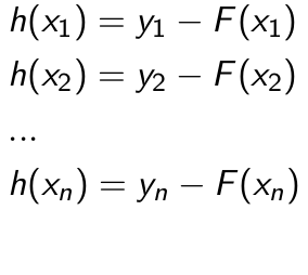
To get h, we fit a model on the points (x1, y1-F(x1)), (x2, y2-F(x2)), …(xn, yn-F(xn)).
The terms (yi-F(xi)) are called residuals. These are the parts where our existing model F cannot do well. The role of h is to compensate the shortcoming of existing model F. If the new model F + h is still not satisfactory, we can add another regression tree.
How is this related to gradient descent?
Gradient Descent
Minimize a function by moving in the opposite direction of the gradient.
Loss function : J = (y − F (x))²/2

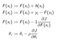
So consider negative gradient is equivalent to residual in case of Gradient Boosting. So, at each step we are trying to reduce residual and in case of Gradient descent we actually travel in the direction of negative gradient and try to reduce loss.
Python Code

n_estimators : int (default=100)
learning_rate : (default=0.1)
max_depth :(default=3) = maximum depth of the individual regression estimators. The maximum depth limits the number of nodes in the tree.
3. XGBoost (Extreme Gradient Boosting)

Do one thing before reading this. Take any recent Kaggle competition, and see top 3 winners approaches. If you don’t find use of XGBoost, shoot me!
Extreme Gradient Boosting (XGBoost) is similar to gradient boosting framework but more efficient. Specifically, XGBoost used a more regularised model formalization to control overfitting, which gives it better performance, which is why it’s also known as ‘regularized boosting‘ technique. It has both linear model solver and tree learning algorithms. Moreover, it has the capacity to do parallel computation on a single machine.
This makes XGBoost at least 10 times faster than existing gradient boosting implementations. It supports various objective functions, including regression, classification and ranking.
Algo Explained:
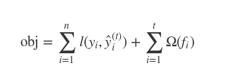
Main difference between GBM and XGBoost is in their objective function. In case of XGBoost Objective Function = Training loss + Regularization
I’m going to leave it here, because explaining Mathematics behind XGBoost will take a completely new blog.
Curiosity is lust of the mind
So, for all the curious mind out there who dwell to explore more! Look here, here and here.
Parameters (Most important for tuning):
**Booster: **You have options like gbtree, gblinear and dart.
**learning_rate: **Similar to learning rate in GBM. Try 0.01–0.2
**max_depth: **Its same as we used in Random Forest, GBM etc. It controls overfitting. Typically values: 3–10
Ohh! these parameters keep repeating themselves **gamma: **Node splitting will be performed only if loss reduction is more than gamma. So, this makes algo conservative.
**lambda and alpha: **Lambda is coefficient of L2 regularization and alpha is for L1 regularization. If you have fear of overfitting, tune these well.
Python code:
Those who are wondering that why I described very few parameters above, I said Important.
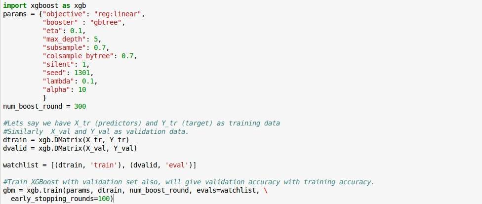

For codes in R, you can refer to this article and for tuning the parameters, you can refer to this one.
Is it really that good?
I like this part of the blogpost the most because at the end, this is what matters. Do keep this in mind!
Pros
Less error based on ensemble method.
Easy to understand.(not for xgboost)
Automatically do feature engineering.
Very little data preparation needed for algorithm.
Suitable if the initial model is pretty bad
Cons
Time and computation expensive.
Complexity of the classification increases.
Hard to implement in real time platform.
Boosting Algorithms generally have 3 parameters which can be fine-tuned, Shrinkage parameter, depth of the tree, the number of trees. Proper training of each of these parameters is needed for a good fit. If parameters are not tuned correctly it may result in over-fitting.
In case of imbalanced dataset, decision trees are biased. However, by using proper splitting criteria, this issue can be resolved.
References
Awesome Resources github repo (IF YOU DON’T OPEN THIS, BLOG WAS NOT WORTH A READ)
AV Blog on Boosting
Kaggle Master Explains Boosting
Sklearn boosting module
Footnotes: One suggestion is that do not miss out references, by reading them only you can understand algorithm properly.
Btw, this completes third algo of our Algorithm series. This is really exciting for us. Cheers!
Hit ❤ if this makes you little bit more intelligent.
Co-author: Gaurav Jindal Editors: Ajay Unagar and Akhil Gupta