ChebNet: CNN on Graphs with Fast Localized Spectral Filtering
Motivation
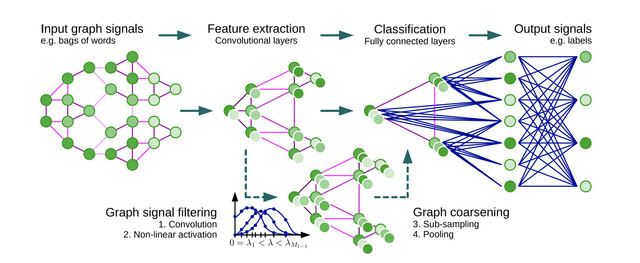
As a part of this blog series, this time we’ll be looking at a spectral convolution technique introduced in the paper by M. Defferrard, X. Bresson, and P. Vandergheynst, on “Convolutional Neural Networks on Graphs with Fast Localized Spectral Filtering”.
As mentioned in our previous blog on A Review : Graph Convolutional Networks (GCN), the spatial convolution and pooling operations are well-defined only for the Euclidean domain. Hence, we cannot apply the convolution directly on the irregular structured data such as graphs.
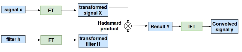
The technique proposed in this paper provide us with a way to perform convolution on graph like data, for which they used convolution theorem. According to which, Convolution in spatial domain is equivalent to multiplication in Fourier domain. Hence, instead of performing convolution explicitly in the spatial domain, we will transform the graph data and the filter into Fourier domain. Do element-wise multiplication and the result is converted back to spatial domain by performing inverse Fourier transform. Following figure illustrates the proposed technique:
But How to Take This Fourier Transform?
As mentioned we have to take a fourier transform of graph signal. In spectral graph theory, the important operator used for Fourier analysis of graph is the Laplacian operator. For the graph G=(V,E), with set of vertices V of size n and set of edges E. The Laplacian is given by
$Δ=D−A$
where D denotes the diagonal degree matrix and A denotes the adjacency matrix of the graph.
When we do eigen-decomposition of the Laplacian, we get the orthonormal eigenvectors, as the Laplacian is real symmetric positive semi-definite matrix (side note: positive semidefinite matrices have orthogonal eigenvectors and symmetric matrix has real eigenvalues). These eigenvectors are denoted by $\phi_{ll=0}^{n}$ and also called as Fourier modes. The corresponding eigenvalues $\lambda_{ll=0}^{n}$ acts as frequencies of the graph.
The Laplacian can be diagonalized by the Fourier basis.
$\Delta = \Phi \Lambda \Phi^T$
where, $\Phi = \phi_{ll=0}^{n}$ is a matrix with eigenvectors as columns and $\Lambda$ is a diagonal matrix of eigenvalues.
Now the graph can be transformed to Fourier domain just by multiplying by the Fourier basis. Hence, the Fourier transform of graph signal x:V→R which is defined on nodes of the graph $x \in \mathbb{R}^n$ is given by:
$\hat{x} = \Phi^T x$, where $\hat{x}$ denotes the graph Fourier transform. Hence, the task of transforming the graph signal to Fourier domain is nothing but the matrix-vector multiplication.
Similarly, the inverse graph Fourier transform is given by: $x = \Phi \hat{x}$. This formulation of Fourier transform on graph gives us the required tools to perform convolution on graphs.
Filtering of Signals on Graph
As we now have the two necessary tools to define convolution on non-Euclidean domain:
-
Way to transform graph to Fourier domain.
-
Convolution in Fourier domain, the convolution operation between graph signal x and filter g is given by the graph convolution of the input signal x with a filter $g \in \mathbb{R}^n$ defined as:
$x *_G g = \mathcal{F}^{-1} \left( \mathcal{F}(x) \odot \mathcal{F}(g) \right) = \Phi \left( \Phi^T x \odot \Phi^T g \right)$,
where ⊙ denotes the element-wise product. If we denote a filter as $g_\theta = \mathrm{diag}(\Phi^T g)$, then the spectral graph convolution is simplified as $x *G g\theta = \Phi g_\theta \Phi^T x$
Why can’t we go forward with this scheme?
All spectral-based ConvGNNs follow this definition. But, this method has three major problems:
-
The number of filter parameters to learn depends on the dimensionality of the input which translates into O(n) complexity and filter is non-parametric.
-
The filters are not localized i.e. filters learnt for graph considers the entire graph, unlike traditional CNN which takes only nearby local pixels to compute convolution.
-
The algorithm needs to calculate the eigen-decomposition explicitly and multiply signal with Fourier basis as there is no Fast Fourier Transform algorithm defined for graphs, hence the computation is $O(n^2)$. (Fast Fourier Transform defined for Euclidean data has $O(nlogn)$ complexity)
Polynomial Parametrization of Filters
To overcome these problems they used an polynomial approximation to parametrize the filter. Now, filter is of the form of: $g_θ(Λ) =\sum_{k=0}^{K-1}θ_kΛ_k$, where the parameter θ∈RK is a vector of polynomial coefficients. These spectral filters represented by Kth-order polynomials of the Laplacian are exactly K-localized. Besides, their learning complexity is O(K), the support size of the filter, and thus the same complexity as classical CNNs.
Is everything fixed now?
No, the cost to filter a signal is still high with $O(n^2)$ operations because of the multiplication with the Fourier basis U. (calculating the eigen-decomposition explicitly and multiply signal with Fourier basis)
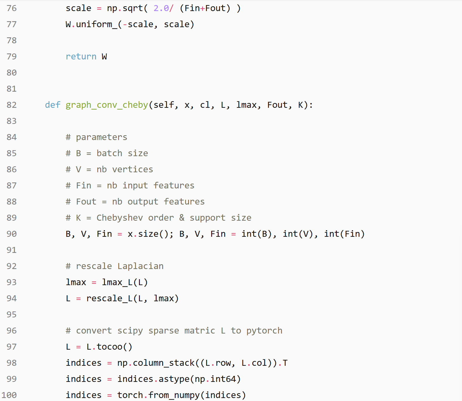
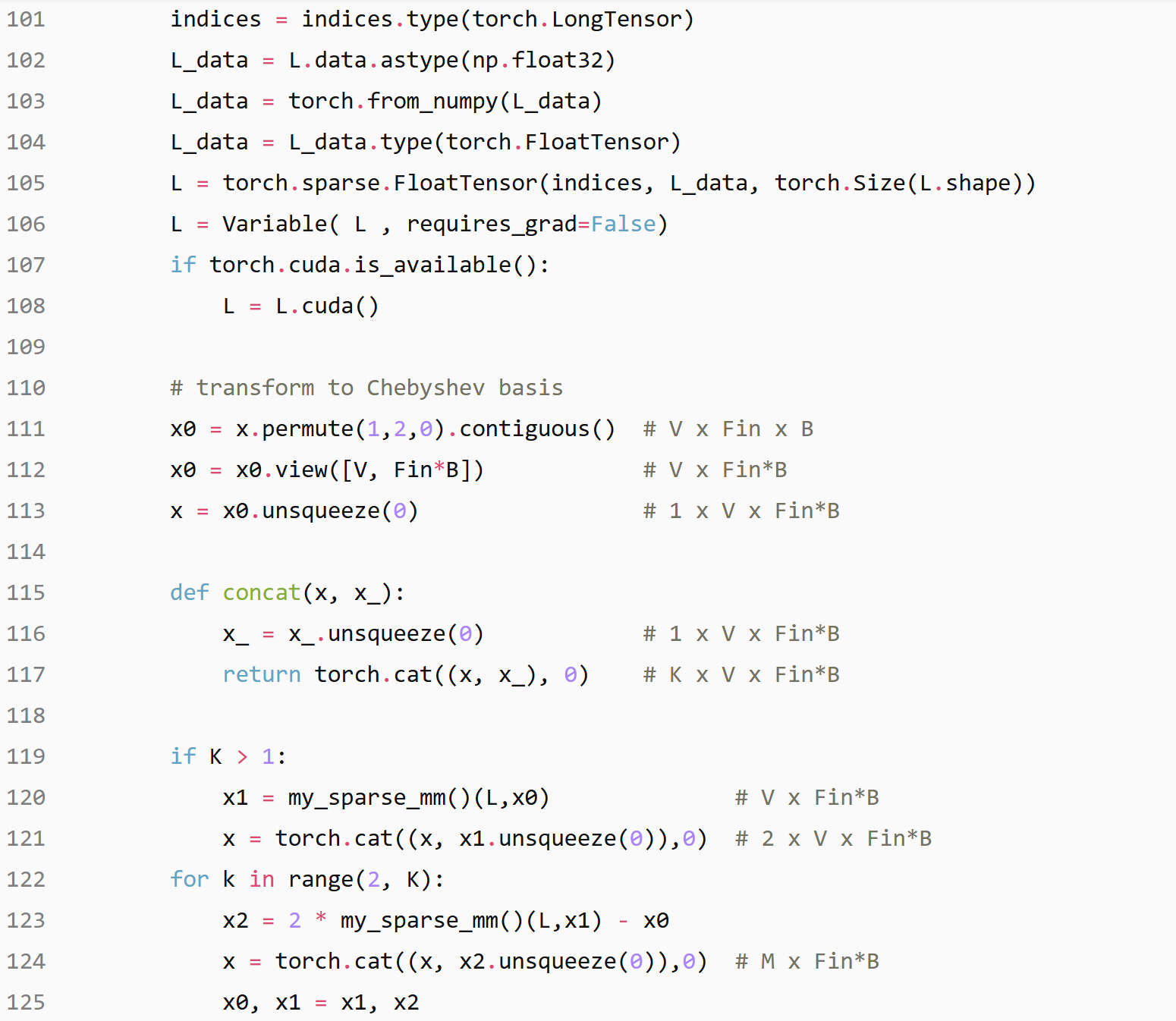
To bypass this problem, the authors parametrize $g_θ(Δ)$) as a polynomial function that can be computed recursively from $Δ$. One such polynomial, traditionally used in Graph Signal Processing to approximate kernels, is the Chebyshev expansion. The Chebyshev polynomial $T_k(x)$ of order k may be computed by the stable recurrence relation $T_k(x) = 2xT_{k−1}(x)−T_{k−2}(x) with $T_0=1$ and $T_1=x$.
The spectral filter is now given by a truncated Chebyshev polynomial: \(g_θ(\barΔ)=Φg(\barΛ)Φ^T=\sum_{k=0}^{K-1}θ_kT_k(\barΔ)\) where, $Θ∈R^K$ now represents a vector of the Chebyshev coefficients, the $\barΔ$ denotes the rescaled $Δ$. (This rescaling is necessary as the Chebyshev polynomial form orthonormal basis in the interval [-1,1] and the eigenvalues of original Laplacian lies in the interval $[0,λ_{max}]$). Scaling is done as $\barΔ= 2Δ/λ_{max}−I_n$.
The filtering operation can now be written as $y=g_θ(Δ)x=\sum_{k=0}^{K-1}θ_kT_k(\barΔ)x$, where, $x_{i,k}$ are the input feature maps, $Θ_k$ are the trainable parameters.
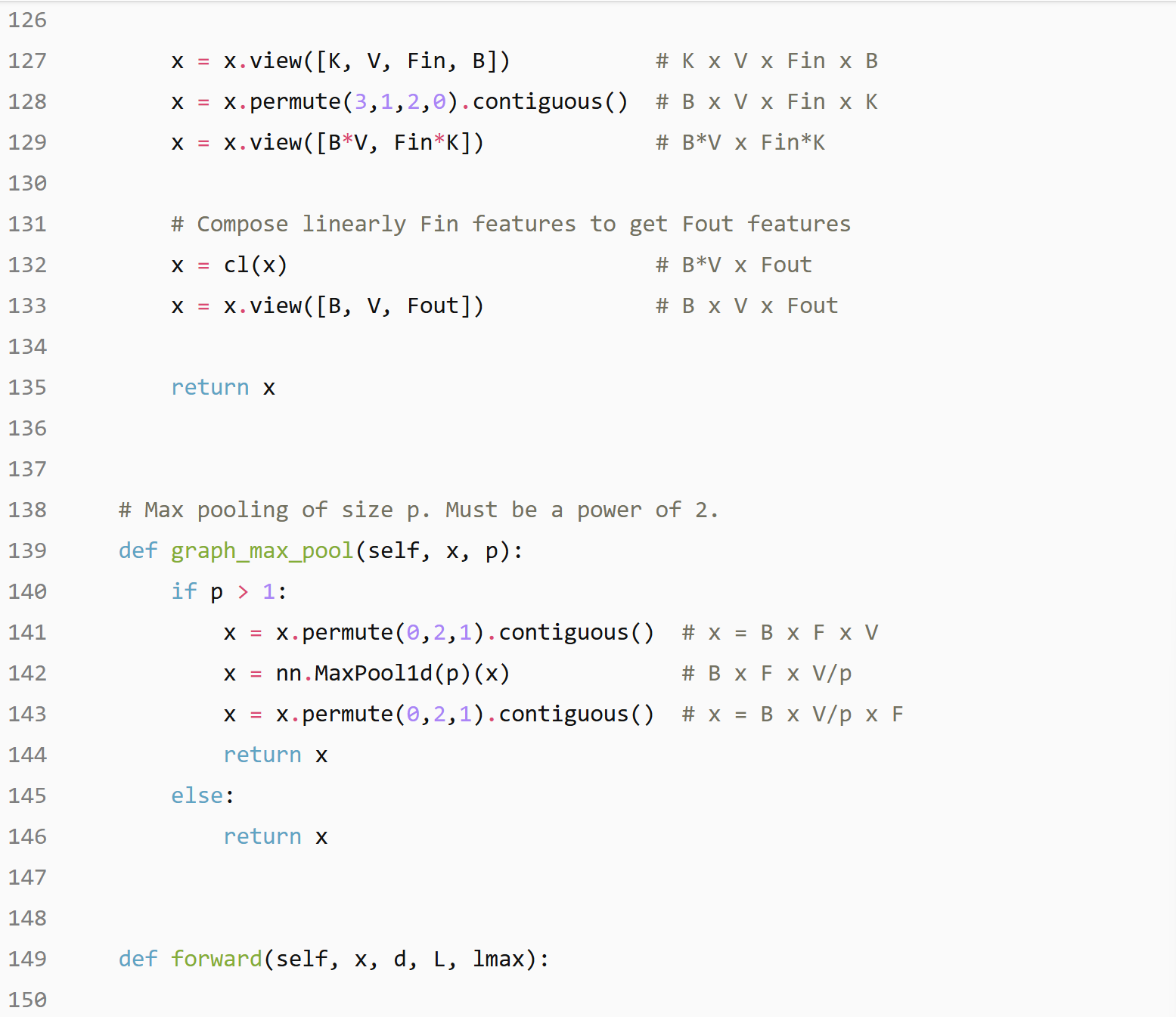
Pooling Operation
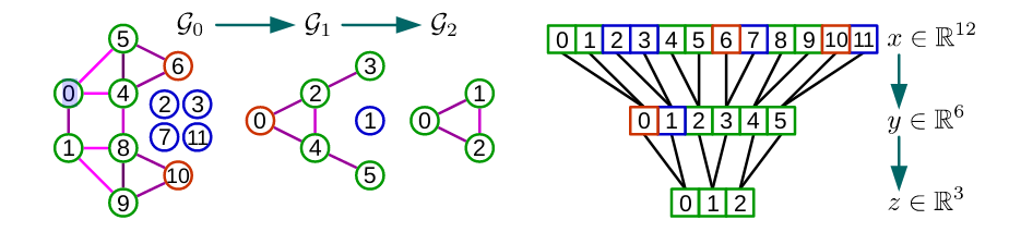
In case of images, the pooling operation consists of taking a fixed size patch of pixels, say 2x2, and keeping only the pixel with max value (assuming you apply max pooling) and discarding the other pixels from the patch. Similar concept of pooling can be applied to graphs.
Defferrard et al. address this issue by using the coarsening phase of the Graclus multilevel clustering algorithm. Graclus’ greedy rule consists, at each coarsening level, in picking an unmarked vertex $i$ and matching it with one of its unmarked neighbors $j$ that maximizes the local normalized cut $Wij(1/di+ 1/dj)$. The two matched vertices are then marked and the coarsened weights are set as the sum of their weights. The matching is repeated until all nodes have been explored. This is an very fast coarsening scheme which divides the number of nodes by approximately two from one level to the next coarser level. After coarsening, the nodes of the input graph and its coarsened version are rearranged into a balanced binary tree. Arbitrarily aggregating the balanced binary tree from bottom to top will arrange similar nodes together. Pooling such a rearranged signal is much more efficient than pooling the original. The following figure shows the example of graph coarsening and pooling.
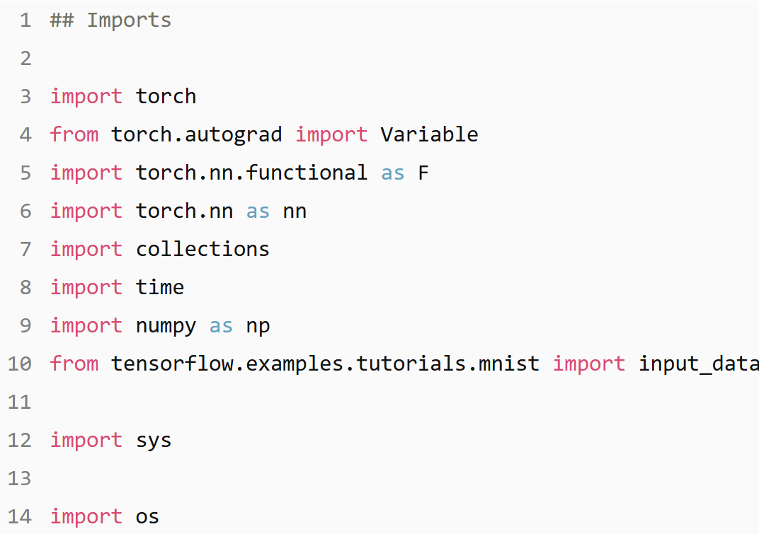
Implementing ChebNET in PyTorch
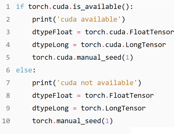 cuda available
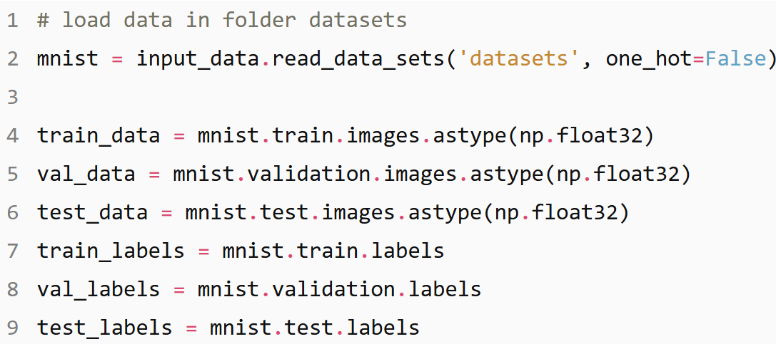
Data Preparation
 nb edges: 6396
 Heavy Edge Matching coarsening with Xavier version
Layer 0: M_0 = |V| = 976 nodes (192 added), |E| = 3198 edges
Layer 1: M_1 = |V| = 488 nodes (83 added), |E| = 1619 edges
Layer 2: M_2 = |V| = 244 nodes (29 added), |E| = 794 edges
Layer 3: M_3 = |V| = 122 nodes (7 added), |E| = 396 edges
Layer 4: M_4 = |V| = 61 nodes (0 added), |E| = 194 edges
Heavy Edge Matching coarsening with Xavier version
Layer 0: M_0 = |V| = 976 nodes (192 added), |E| = 3198 edges
Layer 1: M_1 = |V| = 488 nodes (83 added), |E| = 1619 edges
Layer 2: M_2 = |V| = 244 nodes (29 added), |E| = 794 edges
Layer 3: M_3 = |V| = 122 nodes (7 added), |E| = 396 edges
Layer 4: M_4 = |V| = 61 nodes (0 added), |E| = 194 edges
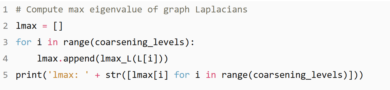 lmax: [1.3857538, 1.3440963, 1.1994357, 1.0239158]
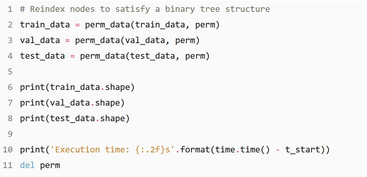 (55000, 976)
(5000, 976)
(10000, 976)
Execution time: 4.18s
(55000, 976)
(5000, 976)
(10000, 976)
Execution time: 4.18s
Model
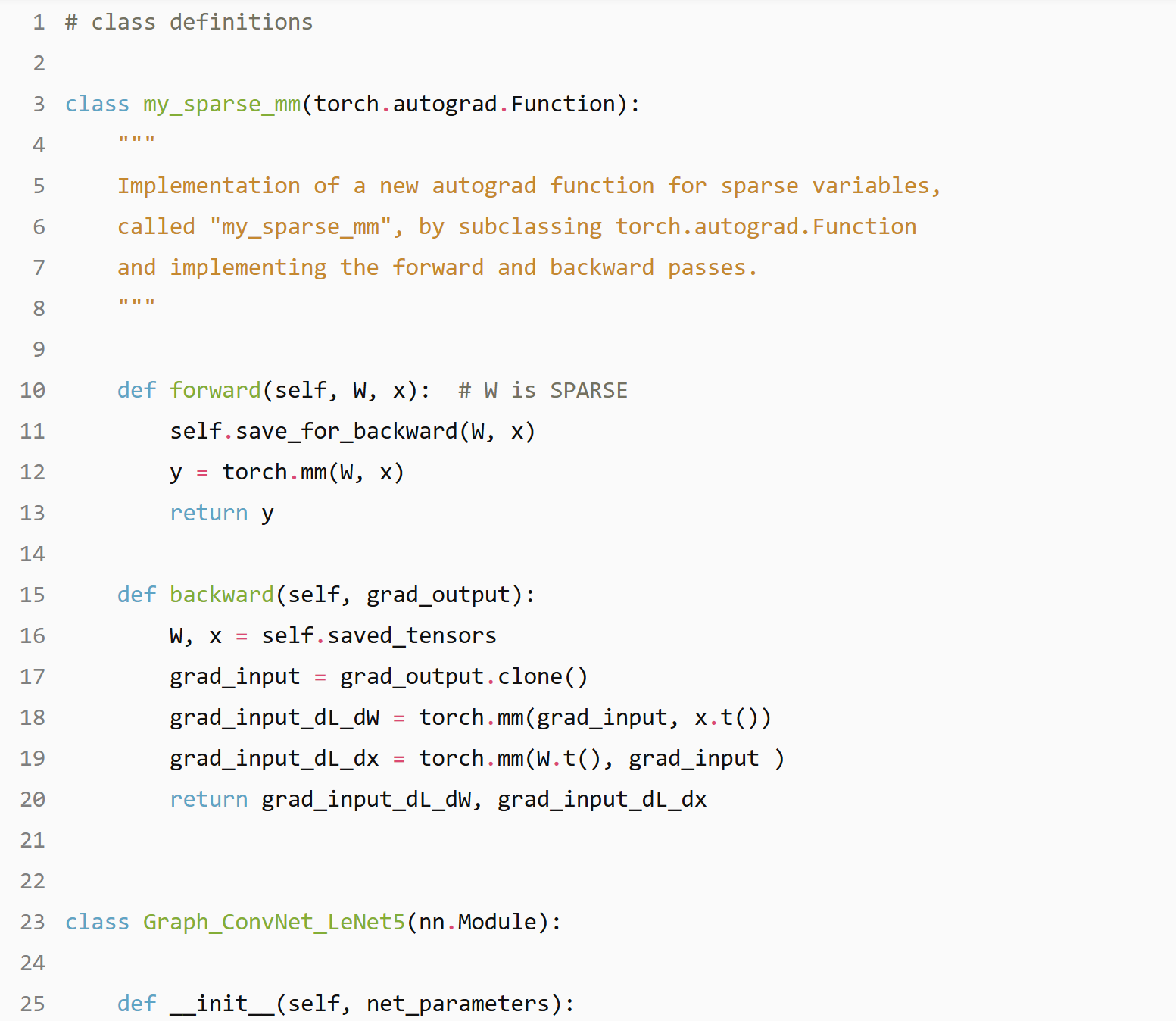
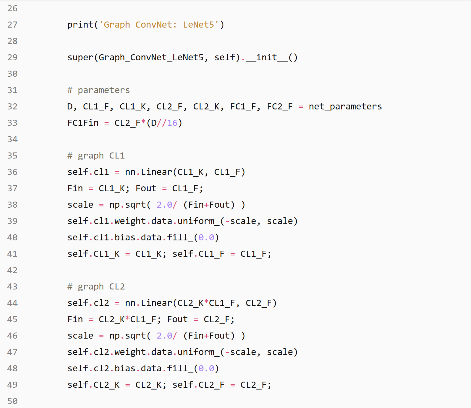
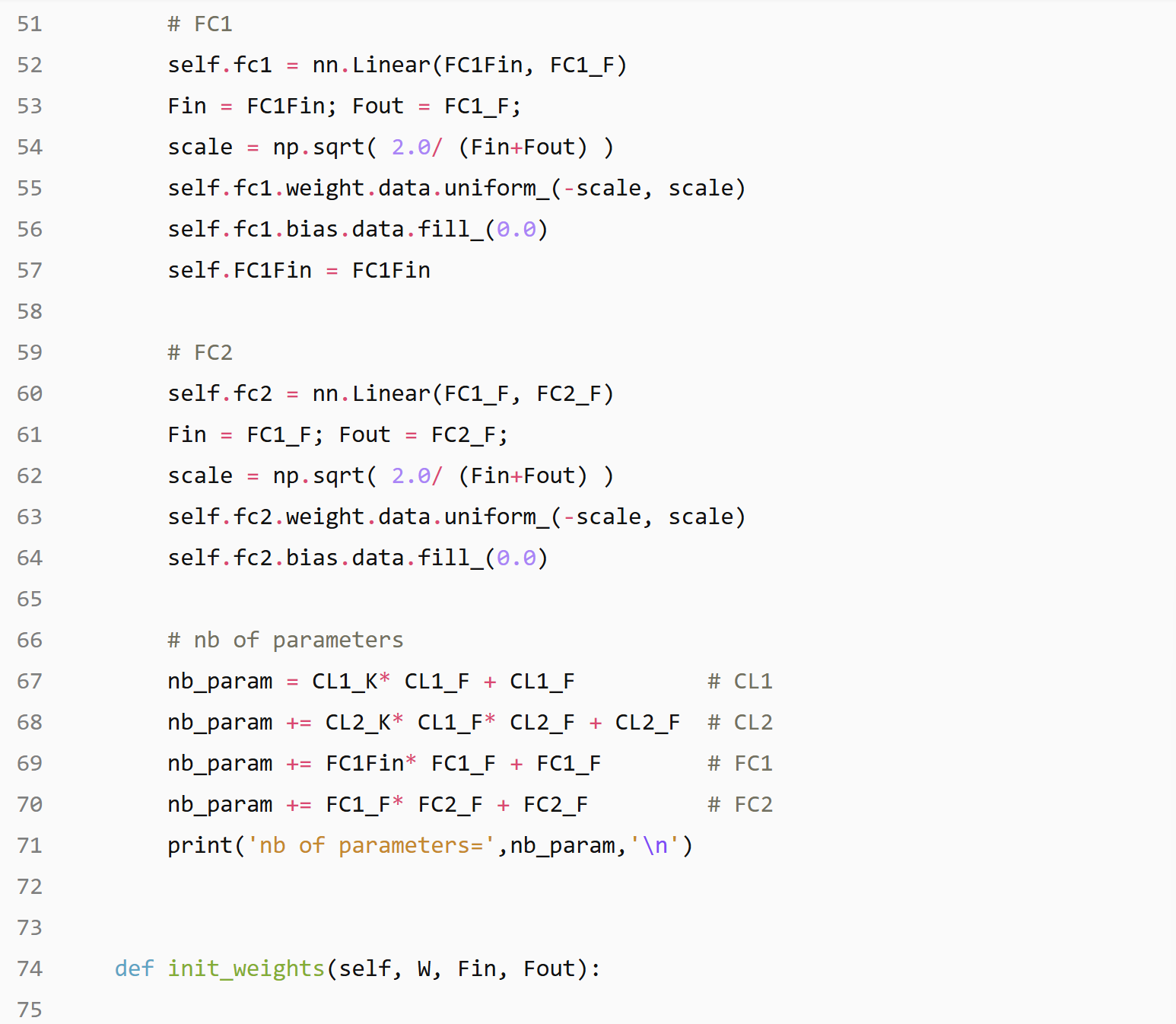
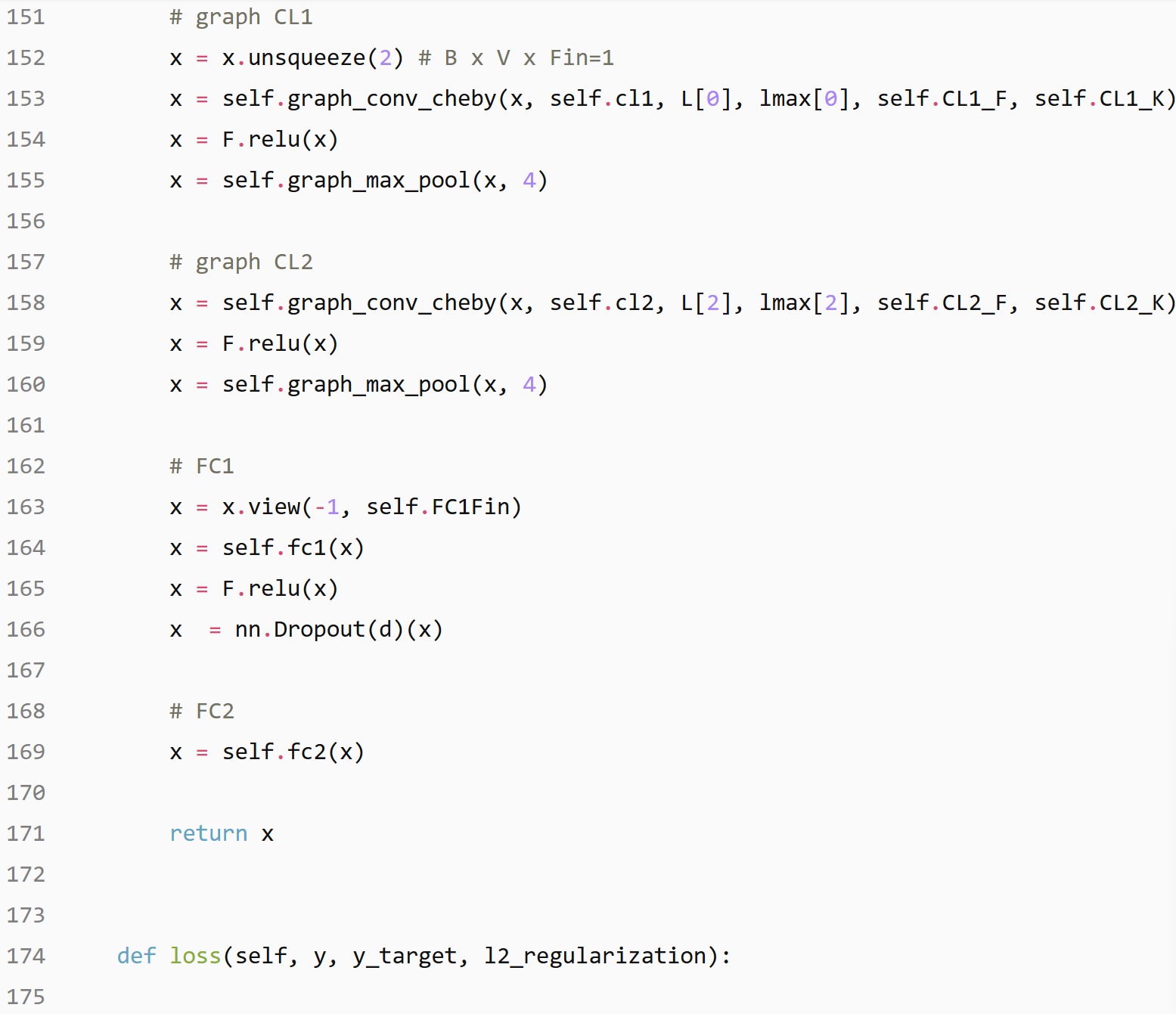
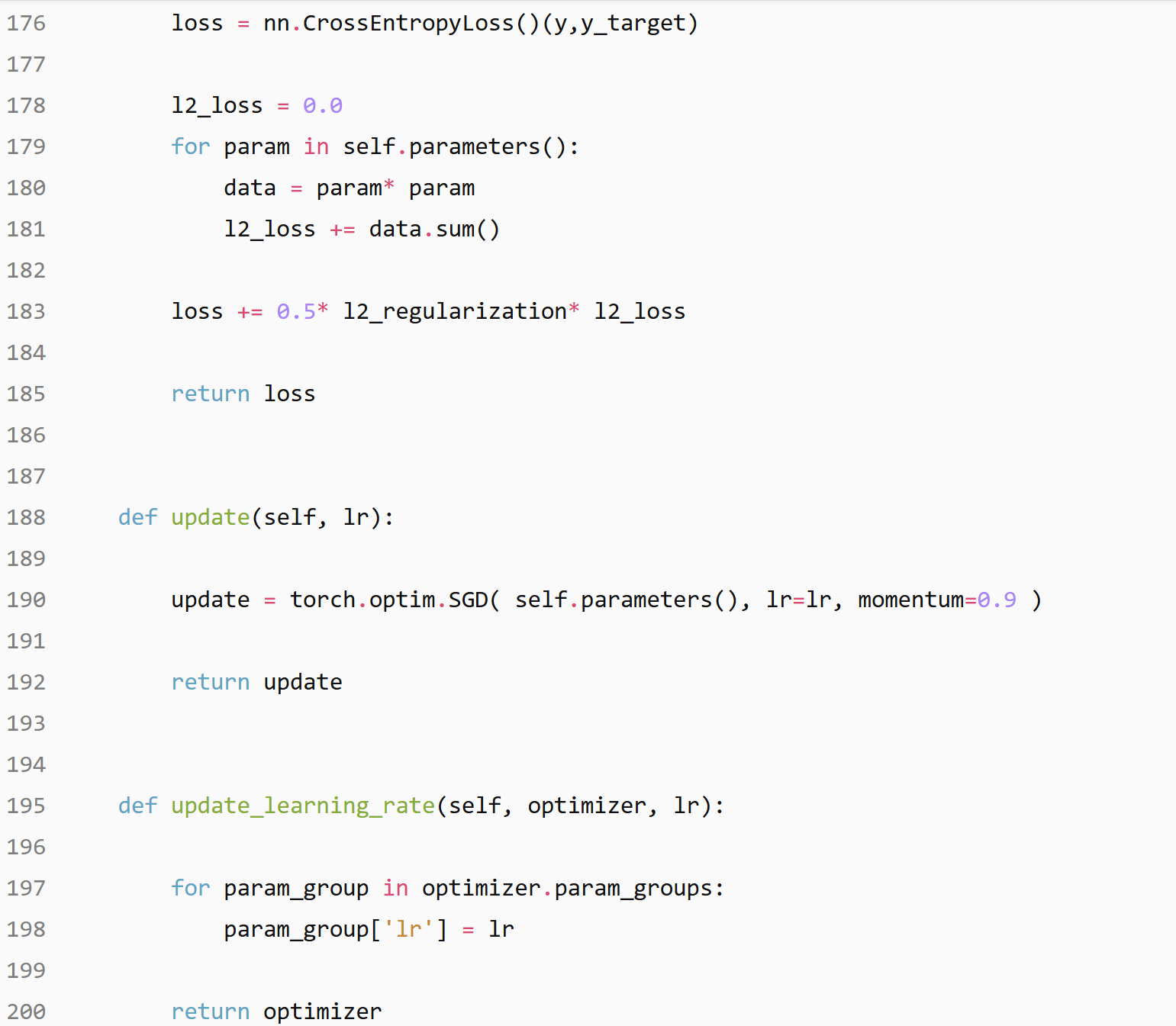
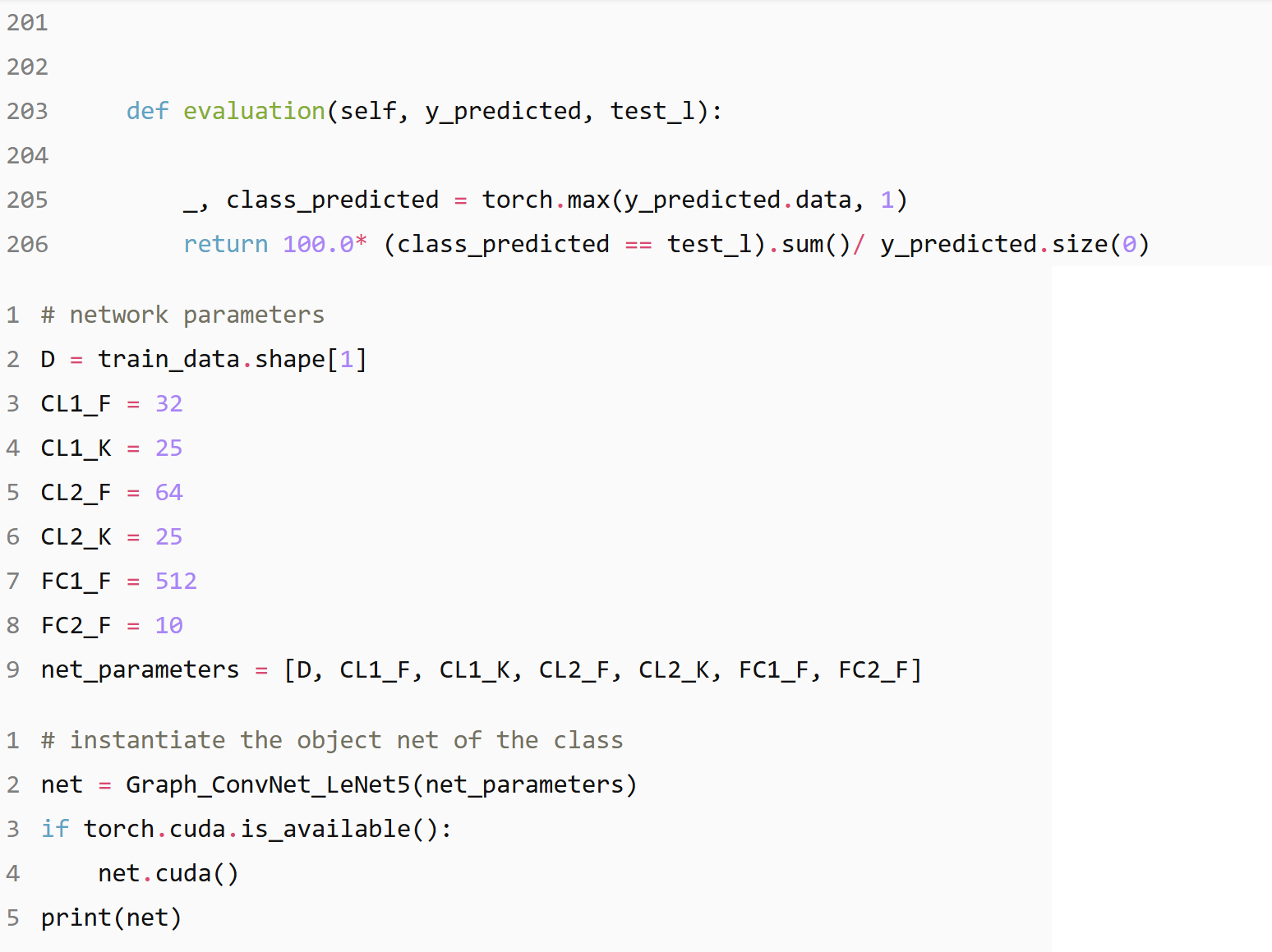 Graph ConvNet: LeNet5
nb of parameters= 2056586
Graph_ConvNet_LeNet5(
(cl1): Linear(in_features=25, out_features=32, bias=True)
(cl2): Linear(in_features=800, out_features=64, bias=True)
(fc1): Linear(in_features=3904, out_features=512, bias=True)
(fc2): Linear(in_features=512, out_features=10, bias=True)
)
Graph ConvNet: LeNet5
nb of parameters= 2056586
Graph_ConvNet_LeNet5(
(cl1): Linear(in_features=25, out_features=32, bias=True)
(cl2): Linear(in_features=800, out_features=64, bias=True)
(fc1): Linear(in_features=3904, out_features=512, bias=True)
(fc2): Linear(in_features=512, out_features=10, bias=True)
)

Hyper parameters setting
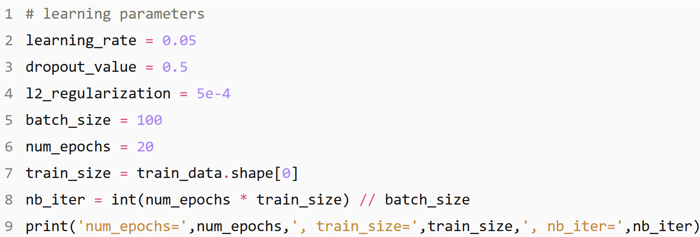 num_epochs= 20 , train_size= 55000 , nb_iter= 11000
Training & Evaluation
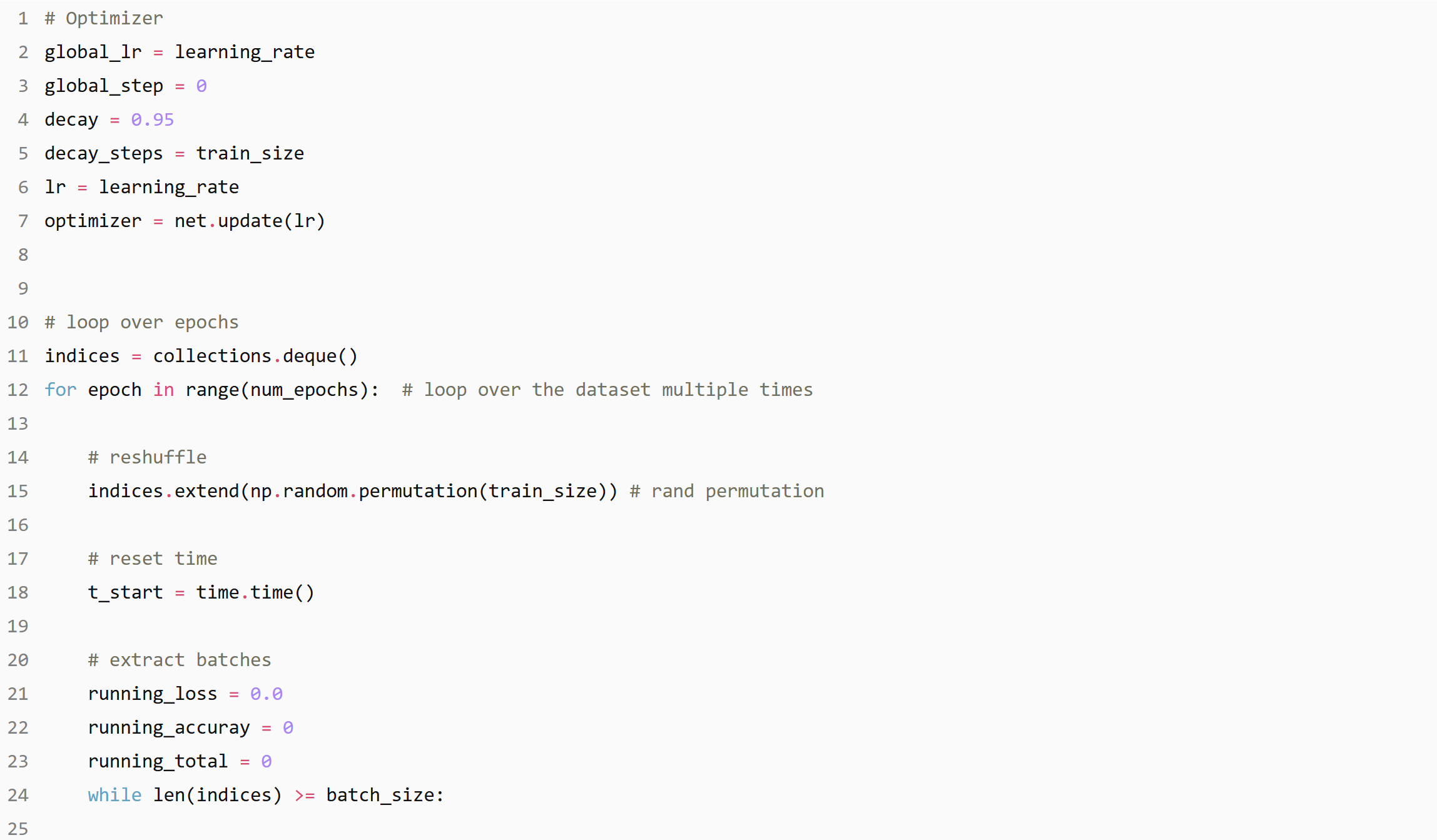
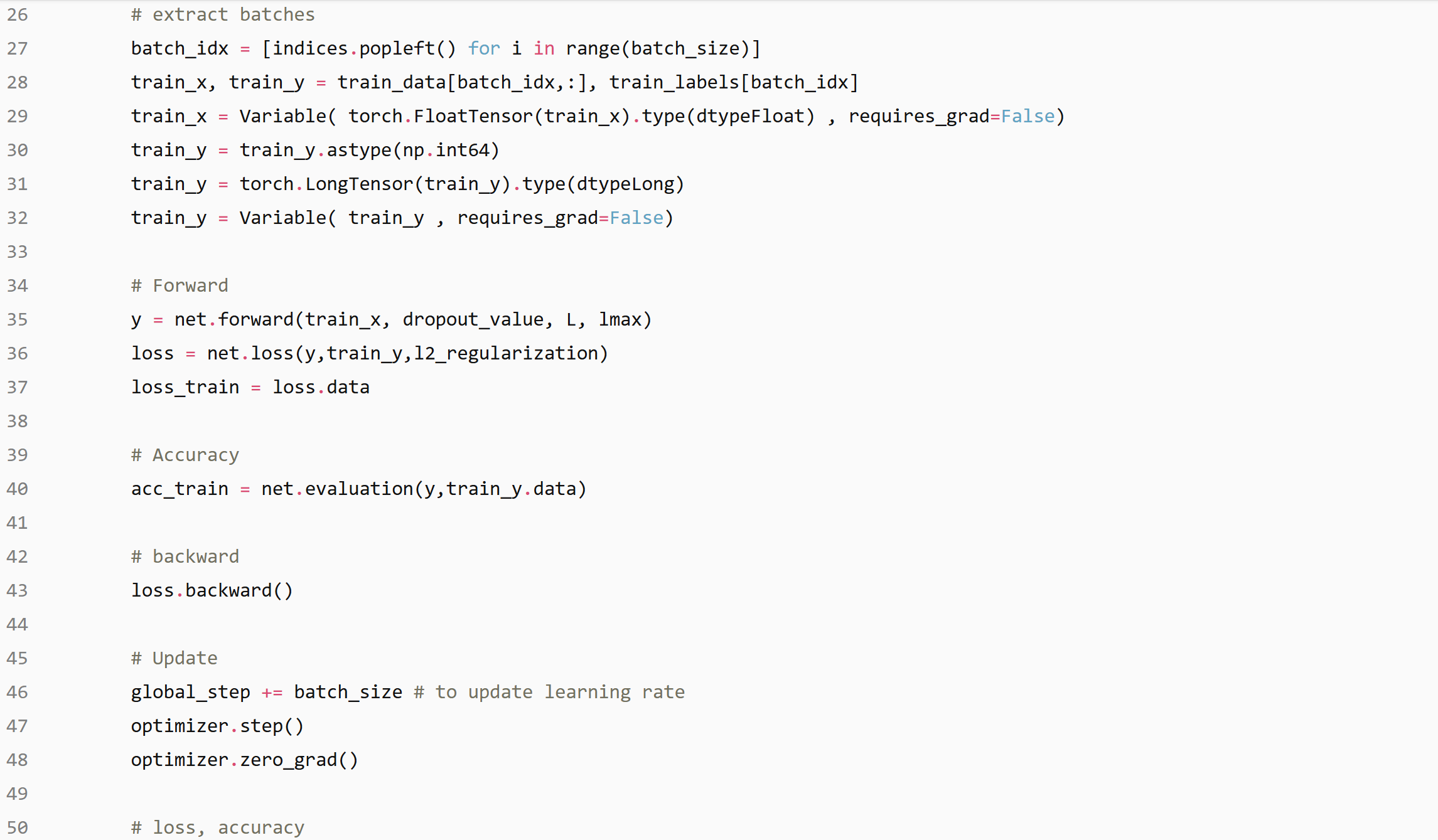
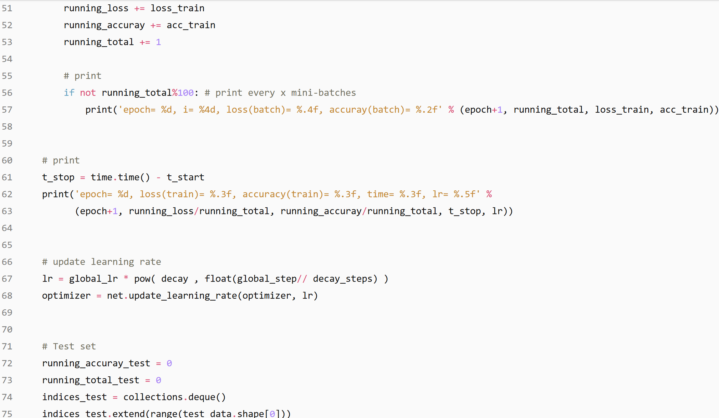
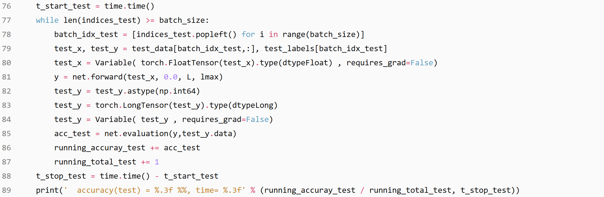
You can find our implementation made using PyTorch at ChebNet.
References
Convolutional Neural Networks on Graphs with Fast Localised Spectral Filtering